
Deep learning CNN Model for predicting Covid-19 from Chest X-ray Images
Table of Contents
Background
Machine learning in diagnosis of Covid-19
What is CNN model?
Architecture of CNN model
Objective
Data structure
Visualizing few images
Importing necessary libraries
Data augmentation
Defining the model
Compiling and training the model
Model evaluation
Predictions, Confusion matrix and ROC_AUC score
Gradient weighted class activation maps
K-fold cross validation
Conclusion
BACKGROUND
Coronaviruses are a group of viruses that cause serious respiratory infections of humans and animals. Covid-19, the recent contagious pandemic disease which shook the whole world is caused by one such Coronavirus, the severe acute respiratory syndrome coronavirus 2 (SARS-CoV-2). The disease is characterized by cold, cough, fever and in the severe form presents as pneumonia of lungs.
MACHINE LEARNING IN DIAGNOSIS OF COVID-19
The foremost step in fighting the disease is to identify the infected patients early enough so as to provide them adequate support and to further prevent the spread. Currently, the gold standard test for diagnosis of Covid-19 is the Reverse transcriptase polymerase chain reaction (RT-PCR). Nevertheless, there are several challenges associated, such as the need of dedicated instruments, need of experienced personnel, the possibility of false negative results and takes at least two days to complete. Thus, there is an alarming need to look for alternative methods for rapid and accurate diagnosis of Covid-19.
In this context, chest radiological imaging in the form of X-rays or Computed tomography (CT), might be helpful. Although, chest CT provides efficient and sensitive diagnosis of Covid-19, it is expensive, uses high levels of radiation and cannot be employed for screening purposes. On the other hand, X-ray is less sensitive than CT, however it is cheaper, faster and best alternative for routine diagnosis. X-rays for Covid-19 are characterized with the presence of multiple, patchy, sub-segmental, or segmental ground glass opacities in the lungs. These subtle patterns can only be identified and interpreted by experienced radiologists. Considering the dearth of trained radiologists and enormous number of suspected individuals, there is an urgent need to develop automatic methods that can identify such abnormalities and assist in the rapid diagnosis of Covid-19. Machine learning or Deep learning algorithms such as Convolutional Neural Networks (CNN), can serve as powerful tools for solving such problems.
WHAT IS CNN MODEL?
CNN is a class of deep learning algorithm, widely used for image classification. Compared to other algorithms, it requires much less pre-processing and can achieve better results with enough training. It is analogous to the neuron operating characteristic of human brain.
ARCHITECTURE OF CNN MODEL
CNN is made up of an input layer, multiple hidden layers and an output layer. The hidden layers include convolutional layers, pooling layers, fully connected layers and activation function layers. The convolution and pooling layers extract features from the input image while the fully connected layer maps the extracted feature into final output, such as classification.
OBJECTIVE
Given the vast application of CNN for image classification, a deep learning model can be built to extract features from the chest x-ray images and eventually aid in detection of Covid-19.
The model for the current study has been built using Python, Keras and Tensorflow. Entire coding has been carried out on Google’s Colab environment with Tesla GPU.
DATA STRUCTURE
Data for the study has been downloaded into google drive as “Data” from the open web source:
Disclaimer: The below link corresponds to version 1, published on 09-06-2020. With the availability of data, the versions get updated. Hence, the users are advised to check the data, the version and modify the code accordingly.
data.mendeley.com
The database consists of 488 augmented chest x-ray images, of which 107, 233 and 148 belong to Covid-19 infected, healthy/normal and pneumonia infected individuals, respectively. The corresponding labels are, ‘CV’, ’N’ and ‘P’. The data has been split using split folders in the ratio of 70:30 as train and validation, respectively.
We will be using Python for implementation
import splitfolders
splitfolders.ratio("/content/drive/MyDrive/Data", output="output", seed=1337, ratio=(0.7, 0.3),group_prefix=None)
Figure 1 : Data Schema for the CNN implementation on Covid Chest XRay Data
Figure 2 : Distribution of image samples in the training and validation data sets
VISUALIZING FEW IMAGES
img_path="/content/drive/MyDrive/Data/CV/covid-19-pneumonia-53.jpg"
img=cv2.imread(img_path)
cv2_imshow(img)

img_path="/content/drive/MyDrive/Data/N/IM-0033-0001-0001.jpeg"
img=cv2.imread(img_path)
cv2_imshow(img)

img_path="/content/drive/MyDrive/Data/P/person28_virus_63.jpeg"
img=cv2.imread(img_path)
cv2_imshow(img)
Figure 3 : Sample Images of Chest X-Ray with Covid, Normal and Pneumonia dipictions
IMPORTING NECESSARY LIBRARIES
from keras_preprocessing.image import ImageDataGenerator
from sklearn.metrics import classification_report, confusion_matrix
from mlxtend.plotting import plot_confusion_matrix
from google.colab.patches import cv2_imshow
from keras_preprocessing import image
from sklearn.metrics import roc_auc_score
from sklearn.model_selection import KFold
from sklearn.model_selection import cross_validate
from sklearn.model_selection import RepeatedKFold, cross_val_score
from keras.wrappers.scikit_learn import KerasClassifier
from keras.preprocessing import image
from keras.layers import MaxPooling2D
from keras.models import Sequential
from keras.models import load_model
from keras.layers import Conv2D
from keras.layers import Flatten
from keras.layers import Dense
import warnings
warnings.filterwarnings('ignore')
from google.colab.patches import cv2_imshow
import cv2
from IPython.display import Image
import matplotlib.pyplot as plt
import tensorflow
import seaborn as sns
from numpy.random import seed
seed(1)
from tensorflow import keras
import keras_preprocessing
from tensorflow import keras
import matplotlib.cm as cm
from numpy.random import seed
from skimage import transform
from PIL import Image
import tensorflow as tf
import numpy as np
import pandas as pd
import h5py
import os
import PIL
import cv2
DATA AUGMENTATION
Training a CNN on limited data results in overfitting and subsequently the model might not generalize well on unseen data. To prevent this, data augmentation techniques such as zoom in and out, cropping, horizontal flipping etc, which can increase the diversity of data can be applied.
train_dir="/content/output/train"
train_datagen=ImageDataGenerator(
    rescale=1./255,
    shear_range=0.2,
    zoom_range=0.2,
    horizontal_flip=True,
    )

val_dir="/content/output/val"
val_datagen=ImageDataGenerator(
    rescale=1./255)

train_generator=train_datagen.flow_from_directory(train_dir,
target_size=(224,224),class_mode='categorical',batch_size=32)

valid_generator=val_datagen.flow_from_directory(val_dir,
target_size=(224,224),class_mode='categorical',batch_size=32,shuffle=False)
DEFINING THE MODEL
A model is defined with four convolutional layers, max-pooling layers, a dropout layer to avoid overfitting and the activation function, Relu, which adds non-linearity to the data is included in the hidden layers. Since the task is a multi-label classification, final output layer includes Softmax function, which predicts the probability of individual classes.
unit=[]
for x in range (0,len(train_generator.class_indices)):
    unit.append(x)

units=x+1
model1 =tf.keras.models.Sequential([
    tf.keras.layers.Conv2D(64,(3,3),activation='relu',input_shape=(224,224,3)),
    tf.keras.layers.MaxPooling2D(2,2),
    tf.keras.layers.Conv2D(64,(3,3),activation='relu'),
    tf.keras.layers.MaxPooling2D(2,2),
    tf.keras.layers.Conv2D(128,(3,3),activation='relu'),
    tf.keras.layers.MaxPooling2D(2,2),
    tf.keras.layers.Conv2D(64,(3,3),activation='relu'),
    tf.keras.layers.MaxPooling2D(2,2),
    tf.keras.layers.Flatten(),
    tf.keras.layers.Dropout(0.5),
    tf.keras.layers.Dense(512,activation='relu'),
    tf.keras.layers.Dense(units=units,activation='softmax')
    ])
COMPILING AND TRAINING THE MODEL
The model is next compiled with Adam optimizer, categorical cross entropy as the loss function and trained for 10 epochs. The evaluation metric used is ‘Accuracy’, defined as the percentage of correct predictions made by the model.
model1.compile(loss='categorical_crossentropy',optimizer='adam',metrics=['accuracy'])
history=model1.fit(train_generator,epochs=10,validation_data=valid_generator)
model1.summary()
MODEL EVALUATION
The model is then evaluated by plotting the loss function and the accuracy of train versus the validation data.
loss_train = history.history['loss']
loss_val = history.history['val_loss']
acc_train = history.history['accuracy']
acc_val = history.history['val_accuracy']

epochs = range(1,11)

plt.figure(figsize=(15, 15))
plt.subplot(2, 2, 1)
plt.plot(epochs, loss_train, 'g', label='Training loss')
plt.plot(epochs, loss_val, 'b', label='Validation loss')
plt.legend(loc='lower left')
plt.title('Training and Validation loss')
plt.xlabel('Epochs')
plt.ylabel('Loss')

plt.subplot(2, 2, 2)
plt.plot(epochs, acc_train, 'g', label='Training accuracy')
plt.plot(epochs, acc_val, 'b', label='Validation accuracy')
plt.legend(loc='lower right')
plt.title('Training and Validation accuracy')
plt.xlabel('Epochs')
plt.ylabel('Accuracy')

plt.show()
At the end of 10 epochs, the model achieves a training accuracy of 0.78 and validation accuracy of 0.86. The training and validation loss was found to be 0.45 and 0.37, respectively. You can observe the parameters w.r.t the epochs in figure 4 below.
Figure 4: Graph of Training Loss Vs Validation Loss along with Training Accuracy Vs Validation Accuracy
PREDICTIONS, CONFUSION MATRIX, CLASSIFICATION REPORT AND ROC_AUC SCORE
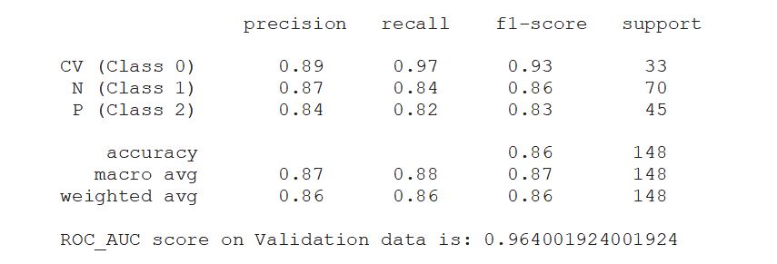
Predictions are then made on validation data and performance of the model is evaluated in terms of accuracy, precision and recall through confusion matrix. ROC_AUC score is another metric used, which measures the ability of the model to distinguish between classes.
Y_pred = model1.predict_generator(valid_generator)
y_pred = np.argmax(Y_pred, axis=1)
conf=confusion_matrix(valid_generator.classes,y_pred)
classnames = ['CV (Class 0)', 'N (Class 1)', 'P (Class 2)']
plt.title('Confusion matrix of Validation data')
sns.heatmap(conf, xticklabels=classnames, yticklabels=classnames, annot=True,cmap="YlGnBu")
plt.xlabel('Predicted')
plt.ylabel('Actual')
plt.show()
print(classification_report(valid_generator.classes, y_pred, target_names=classnames))

y_pred2=model1.predict(valid_generator)
roc_auc=roc_auc_score(valid_generator.classes,y_pred2,multi_class='ovo')
print('ROC_AUC score on Validation data is:',roc_auc)
Figure 5 : Graphical Illustration of CNN models confusion matrix on training and validation data
GRADIENT WEIGHTED CLASS ACTIVATION MAP (Grad-cam)
Grad-cam is a popular technique of making class-specific heatmap by highlighting the regions of input image that the CNN has considered relevant to perform predictions. It helps to visualize the output of a CNN.
last_conv_layer_name = "conv2d_3"
model1_layer_names = [
    'max_pooling2d',
    'max_pooling2d_1',
    'max_pooling2d_2',
    'max_pooling2d_3',
    'flatten',
    'dropout',
    'dense',
   'dense_1'
]
class_index=0


img_path="/content/drive/MyDrive/Data/P/person28_virus_62.jpeg"
img=cv2.imread(img_path)
cv2_imshow(img)
def load(file):
   np_image = Image.open(file)
   np_image = np.array(np_image).astype('float32')/255
   np_image = transform.resize(np_image, (224, 224, 3))
   np_image = np.expand_dims(np_image, axis=0)
   return np_image

myfile="/content/drive/MyDrive/Data/P/person28_virus_62.jpeg"
image = load(myfile)
print(model1.predict(image))

gradient_model = tf.keras.models.Model([model1.inputs],
                                                                   [model1.get_layer(last_conv_layer_name).output, model1.output])

with tf.GradientTape() as tape:
    convol_outputs, predictions = gradient_model(image)
    loss = predictions[:, class_index]

output = convol_outputs
single_grads = tape.gradient(loss, convol_outputs)
pool_grads = tf.reduce_mean(single_grads, axis=(0, 1, 2))
last_conv_layer_output = output.numpy()[0]
pool_grads = pool_grads.numpy()

for i in range(pool_grads.shape[-1]):
        last_conv_layer_output[:, :, i] *= pool_grads[i]
        heat_map = np.mean(last_conv_layer_output, axis=-1)
        heat_map = np.maximum(heat_map, 0) / np.max(heat_map)
plt.matshow(heat_map)
plt.show()

# Loading the original image
img_path="/content/drive/MyDrive/Data/P/person28_virus_62.jpeg"
img = keras.preprocessing.image.load_img(img_path)
img = keras.preprocessing.image.img_to_array(img)

heat_map = np.uint8(255 * heat_map)
jet = cm.get_cmap("jet")
jet_colors = jet(np.arange(256))[:, :3]
jet_heat_map = jet_colors[heat_map]
jet_heat_map = keras.preprocessing.image.array_to_img(jet_heat_map)
jet_heat_map = jet_heat_map.resize((img.shape[1], img.shape[0]))
jet_heat_map = keras.preprocessing.image.img_to_array(jet_heat_map)

# Superimposing the heatmap on original image
superimposed = jet_heat_map * 0.4 + img
superimposed = keras.preprocessing.image.array_to_img(superimposed)
superimposed
Figure 6 : Class Specific Heat Map using Grad-cam
K-FOLD CROSS VALIDATION
Cross-validation is an important technique to assess the performance of a model. In k-fold cross validation, the data is split into k folds and each fold is used as a test set by the model to make predictions.
labels = ['CV', 'N','P']
img_size = 224

def fetch_data(dir):
    data = []
    for label in labels:
        path = os.path.join(dir, label)
        class_num = labels.index(label)
        for img in os.listdir(path):
            try:
                img_arr = cv2.imread(os.path.join(path, img))[...,::-1]
                resized_arr = cv2.resize(img_arr, (img_size, img_size))
                data.append([resized_arr, class_num])
            except Exception as e:
                print(e)
    return np.array(data)

data=fetch_data("/content/drive/MyDrive/Data")
a = []
b = []

for feature, label in data:
  a.append(feature)
  b.append(label)

# Data Normalization
a = np.array(x) / 255
a.reshape(-1, img_size, img_size, 1)

def get_model():
  model =tf.keras.models.Sequential([
    tf.keras.layers.Conv2D(64,(3,3),activation='relu',input_shape=(224,224,3)),
    tf.keras.layers.MaxPooling2D(2,2),
    tf.keras.layers.Conv2D(64,(3,3),activation='relu'),
    tf.keras.layers.MaxPooling2D(2,2),
    tf.keras.layers.Conv2D(128,(3,3),activation='relu'),
    tf.keras.layers.MaxPooling2D(2,2),
    tf.keras.layers.Conv2D(64,(3,3),activation='relu'),
    tf.keras.layers.MaxPooling2D(2,2),
    tf.keras.layers.Flatten(),
    tf.keras.layers.Dropout(0.5),
    tf.keras.layers.Dense(512,activation='relu'),
    tf.keras.layers.Dense(3,activation='softmax')
    ])

  model.compile(loss='categorical_crossentropy',optimizer='adam',metrics=['accuracy'])
  return(model)


Classifier= KerasClassifier(build_fn=get_model, epochs=10, batch_size=10, verbose=0)
kfold= KFold(n_splits=6)
precision= cross_val_score(Classifier, a, b, scoring='precision_micro',cv=kfold)
print('Precision is:',precision)
accuracy= cross_val_score(Classifier, a, b, scoring='accuracy',cv=kfold)
print('Accuracy is:',accuracy)
recall= cross_val_score(Classifier, a, b, scoring='recall_micro',cv=kfold)
print('Recall is:',recall)
f1= cross_val_score(estimator, x, y, scoring='f1_micro',cv=kfold)
print('F1 score is:',f1)
Figure 7 : K fold cross validation metrics
Using 6 folds cross validation, the model achieved 79% precision, 71% accuracy, 76% recall and 77% score, on average over different folds.
CONCLUSION
In conclusion, the proposed model looks promising in identifying and distinguishing Covid-19 from the other two classes of healthy and pneumonia. However, the major limitation of the study is the limited sample size, addressing this problem along with tuning of certain other hyper parameters can further enhance the performance of the model.
About the Author:
Annapurna Satti
Annapurna Satti, an accomplished Life Sciences professional, is an Alumni of University of Hyderabad. She has more than 15 years of research and development (R&D) experience in eminent academic institutes such as Center for DNA Fingerprinting and Diagnostics (CDFD) and Center for Cellular and Molecular Biology (CCMB). As a machine learning enthusiast, she aims to leverage Artificial Intelligence (AI) tools to boost and accelerate research in the field of biotechnology.
Mohan Rai
Mohan Rai is an Alumni of IIM Bangalore , he has completed his MBA from University of Pune and Bachelor of Science (Statistics) from University of Pune. He is a Certified Data Scientist by EMC.Mohan is a learner and has been enriching his experience throughout his career by exposing himself to several opportunities in the capacity of an Advisor, Consultant and a Business Owner. He has more than 18 years’ experience in the field of Analytics and has worked as an Analytics SME on domains ranging from IT, Banking, Construction, Real Estate, Automobile, Component Manufacturing and Retail. His functional scope covers areas including Training, Research, Sales, Market Research, Sales Planning, and Market Strategy.
Table of Contents
- Background
- Machine learning in diagnosis of Covid-19
- What is CNN model?
- Architecture of CNN model
- Objective
- Data structure
- Visualizing few images
- Importing necessary libraries
- Data augmentation
- Defining the model
- Compiling and training the model
- Model evaluation
- Predictions, Confusion matrix and ROC_AUC score
- Gradient weighted class activation maps
- K-fold cross validation
- Conclusion
Coronaviruses are a group of viruses that cause serious respiratory infections of humans and animals. Covid-19, the recent contagious pandemic disease which shook the whole world is caused by one such Coronavirus, the severe acute respiratory syndrome coronavirus 2 (SARS-CoV-2). The disease is characterized by cold, cough, fever and in the severe form presents as pneumonia of lungs.
The foremost step in fighting the disease is to identify the infected patients early enough so as to provide them adequate support and to further prevent the spread. Currently, the gold standard test for diagnosis of Covid-19 is the Reverse transcriptase polymerase chain reaction (RT-PCR). Nevertheless, there are several challenges associated, such as the need of dedicated instruments, need of experienced personnel, the possibility of false negative results and takes at least two days to complete. Thus, there is an alarming need to look for alternative methods for rapid and accurate diagnosis of Covid-19.
In this context, chest radiological imaging in the form of X-rays or Computed tomography (CT), might be helpful. Although, chest CT provides efficient and sensitive diagnosis of Covid-19, it is expensive, uses high levels of radiation and cannot be employed for screening purposes. On the other hand, X-ray is less sensitive than CT, however it is cheaper, faster and best alternative for routine diagnosis. X-rays for Covid-19 are characterized with the presence of multiple, patchy, sub-segmental, or segmental ground glass opacities in the lungs. These subtle patterns can only be identified and interpreted by experienced radiologists. Considering the dearth of trained radiologists and enormous number of suspected individuals, there is an urgent need to develop automatic methods that can identify such abnormalities and assist in the rapid diagnosis of Covid-19. Machine learning or Deep learning algorithms such as Convolutional Neural Networks (CNN), can serve as powerful tools for solving such problems.
CNN is a class of deep learning algorithm, widely used for image classification. Compared to other algorithms, it requires much less pre-processing and can achieve better results with enough training. It is analogous to the neuron operating characteristic of human brain.
CNN is made up of an input layer, multiple hidden layers and an output layer. The hidden layers include convolutional layers, pooling layers, fully connected layers and activation function layers. The convolution and pooling layers extract features from the input image while the fully connected layer maps the extracted feature into final output, such as classification.
Given the vast application of CNN for image classification, a deep learning model can be built to extract features from the chest x-ray images and eventually aid in detection of Covid-19.
The model for the current study has been built using Python, Keras and Tensorflow. Entire coding has been carried out on Google’s Colab environment with Tesla GPU.
Data for the study has been downloaded into google drive as “Data” from the open web source:
Disclaimer: The below link corresponds to version 1, published on 09-06-2020. With the availability of data, the versions get updated. Hence, the users are advised to check the data, the version and modify the code accordingly.
data.mendeley.com
The database consists of 488 augmented chest x-ray images, of which 107, 233 and 148 belong to Covid-19 infected, healthy/normal and pneumonia infected individuals, respectively. The corresponding labels are, ‘CV’, ’N’ and ‘P’. The data has been split using split folders in the ratio of 70:30 as train and validation, respectively.
We will be using Python for implementation
import splitfolders
splitfolders.ratio("/content/drive/MyDrive/Data", output="output", seed=1337, ratio=(0.7, 0.3),group_prefix=None)
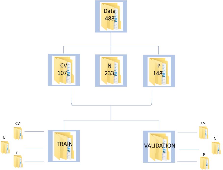
Figure 1 : Data Schema for the CNN implementation on Covid Chest XRay Data
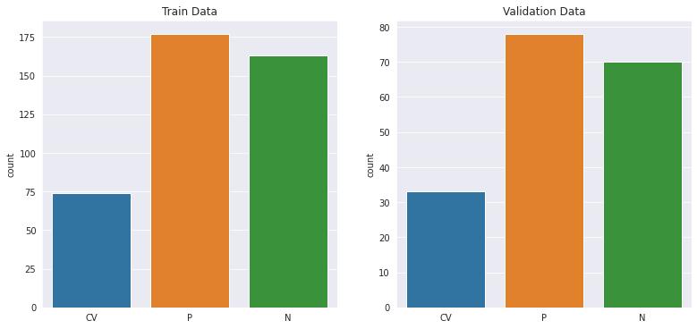
Figure 2 : Distribution of image samples in the training and validation data sets
img_path="/content/drive/MyDrive/Data/CV/covid-19-pneumonia-53.jpg"
img=cv2.imread(img_path)
cv2_imshow(img)
img_path="/content/drive/MyDrive/Data/N/IM-0033-0001-0001.jpeg"
img=cv2.imread(img_path)
cv2_imshow(img)
img_path="/content/drive/MyDrive/Data/P/person28_virus_63.jpeg"
img=cv2.imread(img_path)
cv2_imshow(img)
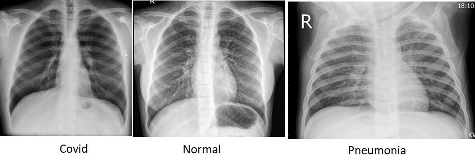
Figure 3 : Sample Images of Chest X-Ray with Covid, Normal and Pneumonia dipictions
from keras_preprocessing.image import ImageDataGenerator
from sklearn.metrics import classification_report, confusion_matrix
from mlxtend.plotting import plot_confusion_matrix
from google.colab.patches import cv2_imshow
from keras_preprocessing import image
from sklearn.metrics import roc_auc_score
from sklearn.model_selection import KFold
from sklearn.model_selection import cross_validate
from sklearn.model_selection import RepeatedKFold, cross_val_score
from keras.wrappers.scikit_learn import KerasClassifier
from keras.preprocessing import image
from keras.layers import MaxPooling2D
from keras.models import Sequential
from keras.models import load_model
from keras.layers import Conv2D
from keras.layers import Flatten
from keras.layers import Dense
import warnings
warnings.filterwarnings('ignore')
from google.colab.patches import cv2_imshow
import cv2
from IPython.display import Image
import matplotlib.pyplot as plt
import tensorflow
import seaborn as sns
from numpy.random import seed
seed(1)
from tensorflow import keras
import keras_preprocessing
from tensorflow import keras
import matplotlib.cm as cm
from numpy.random import seed
from skimage import transform
from PIL import Image
import tensorflow as tf
import numpy as np
import pandas as pd
import h5py
import os
import PIL
import cv2
Training a CNN on limited data results in overfitting and subsequently the model might not generalize well on unseen data. To prevent this, data augmentation techniques such as zoom in and out, cropping, horizontal flipping etc, which can increase the diversity of data can be applied.
train_dir="/content/output/train"
train_datagen=ImageDataGenerator(
rescale=1./255,
shear_range=0.2,
zoom_range=0.2,
horizontal_flip=True,
)
val_dir="/content/output/val"
val_datagen=ImageDataGenerator(
rescale=1./255)
train_generator=train_datagen.flow_from_directory(train_dir,
target_size=(224,224),class_mode='categorical',batch_size=32)
valid_generator=val_datagen.flow_from_directory(val_dir,
target_size=(224,224),class_mode='categorical',batch_size=32,shuffle=False)
A model is defined with four convolutional layers, max-pooling layers, a dropout layer to avoid overfitting and the activation function, Relu, which adds non-linearity to the data is included in the hidden layers. Since the task is a multi-label classification, final output layer includes Softmax function, which predicts the probability of individual classes.
unit=[]
for x in range (0,len(train_generator.class_indices)):
unit.append(x)
units=x+1
model1 =tf.keras.models.Sequential([
tf.keras.layers.Conv2D(64,(3,3),activation='relu',input_shape=(224,224,3)),
tf.keras.layers.MaxPooling2D(2,2),
tf.keras.layers.Conv2D(64,(3,3),activation='relu'),
tf.keras.layers.MaxPooling2D(2,2),
tf.keras.layers.Conv2D(128,(3,3),activation='relu'),
tf.keras.layers.MaxPooling2D(2,2),
tf.keras.layers.Conv2D(64,(3,3),activation='relu'),
tf.keras.layers.MaxPooling2D(2,2),
tf.keras.layers.Flatten(),
tf.keras.layers.Dropout(0.5),
tf.keras.layers.Dense(512,activation='relu'),
tf.keras.layers.Dense(units=units,activation='softmax')
])
The model is next compiled with Adam optimizer, categorical cross entropy as the loss function and trained for 10 epochs. The evaluation metric used is ‘Accuracy’, defined as the percentage of correct predictions made by the model.
model1.compile(loss='categorical_crossentropy',optimizer='adam',metrics=['accuracy'])
history=model1.fit(train_generator,epochs=10,validation_data=valid_generator)
model1.summary()
The model is then evaluated by plotting the loss function and the accuracy of train versus the validation data.
loss_train = history.history['loss']
loss_val = history.history['val_loss']
acc_train = history.history['accuracy']
acc_val = history.history['val_accuracy']
epochs = range(1,11)
plt.figure(figsize=(15, 15))
plt.subplot(2, 2, 1)
plt.plot(epochs, loss_train, 'g', label='Training loss')
plt.plot(epochs, loss_val, 'b', label='Validation loss')
plt.legend(loc='lower left')
plt.title('Training and Validation loss')
plt.xlabel('Epochs')
plt.ylabel('Loss')
plt.subplot(2, 2, 2)
plt.plot(epochs, acc_train, 'g', label='Training accuracy')
plt.plot(epochs, acc_val, 'b', label='Validation accuracy')
plt.legend(loc='lower right')
plt.title('Training and Validation accuracy')
plt.xlabel('Epochs')
plt.ylabel('Accuracy')
plt.show()
At the end of 10 epochs, the model achieves a training accuracy of 0.78 and validation accuracy of 0.86. The training and validation loss was found to be 0.45 and 0.37, respectively. You can observe the parameters w.r.t the epochs in figure 4 below.
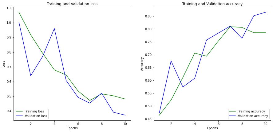
Figure 4: Graph of Training Loss Vs Validation Loss along with Training Accuracy Vs Validation Accuracy
Predictions are then made on validation data and performance of the model is evaluated in terms of accuracy, precision and recall through confusion matrix. ROC_AUC score is another metric used, which measures the ability of the model to distinguish between classes.
Y_pred = model1.predict_generator(valid_generator)
y_pred = np.argmax(Y_pred, axis=1)
conf=confusion_matrix(valid_generator.classes,y_pred)
classnames = ['CV (Class 0)', 'N (Class 1)', 'P (Class 2)']
plt.title('Confusion matrix of Validation data')
sns.heatmap(conf, xticklabels=classnames, yticklabels=classnames, annot=True,cmap="YlGnBu")
plt.xlabel('Predicted')
plt.ylabel('Actual')
plt.show()
print(classification_report(valid_generator.classes, y_pred, target_names=classnames))
y_pred2=model1.predict(valid_generator)
roc_auc=roc_auc_score(valid_generator.classes,y_pred2,multi_class='ovo')
print('ROC_AUC score on Validation data is:',roc_auc)
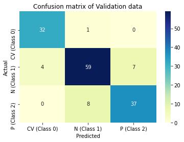
Figure 5 : Graphical Illustration of CNN models confusion matrix on training and validation data
Grad-cam is a popular technique of making class-specific heatmap by highlighting the regions of input image that the CNN has considered relevant to perform predictions. It helps to visualize the output of a CNN.
last_conv_layer_name = "conv2d_3"
model1_layer_names = [
'max_pooling2d',
'max_pooling2d_1',
'max_pooling2d_2',
'max_pooling2d_3',
'flatten',
'dropout',
'dense',
'dense_1'
]
class_index=0
img_path="/content/drive/MyDrive/Data/P/person28_virus_62.jpeg"
img=cv2.imread(img_path)
cv2_imshow(img)
def load(file):
np_image = Image.open(file)
np_image = np.array(np_image).astype('float32')/255
np_image = transform.resize(np_image, (224, 224, 3))
np_image = np.expand_dims(np_image, axis=0)
return np_image
myfile="/content/drive/MyDrive/Data/P/person28_virus_62.jpeg"
image = load(myfile)
print(model1.predict(image))
gradient_model = tf.keras.models.Model([model1.inputs],
[model1.get_layer(last_conv_layer_name).output, model1.output])
with tf.GradientTape() as tape:
convol_outputs, predictions = gradient_model(image)
loss = predictions[:, class_index]
output = convol_outputs
single_grads = tape.gradient(loss, convol_outputs)
pool_grads = tf.reduce_mean(single_grads, axis=(0, 1, 2))
last_conv_layer_output = output.numpy()[0]
pool_grads = pool_grads.numpy()
for i in range(pool_grads.shape[-1]):
last_conv_layer_output[:, :, i] *= pool_grads[i]
heat_map = np.mean(last_conv_layer_output, axis=-1)
heat_map = np.maximum(heat_map, 0) / np.max(heat_map)
plt.matshow(heat_map)
plt.show()
# Loading the original image
img_path="/content/drive/MyDrive/Data/P/person28_virus_62.jpeg"
img = keras.preprocessing.image.load_img(img_path)
img = keras.preprocessing.image.img_to_array(img)
heat_map = np.uint8(255 * heat_map)
jet = cm.get_cmap("jet")
jet_colors = jet(np.arange(256))[:, :3]
jet_heat_map = jet_colors[heat_map]
jet_heat_map = keras.preprocessing.image.array_to_img(jet_heat_map)
jet_heat_map = jet_heat_map.resize((img.shape[1], img.shape[0]))
jet_heat_map = keras.preprocessing.image.img_to_array(jet_heat_map)
# Superimposing the heatmap on original image
superimposed = jet_heat_map * 0.4 + img
superimposed = keras.preprocessing.image.array_to_img(superimposed)
superimposed
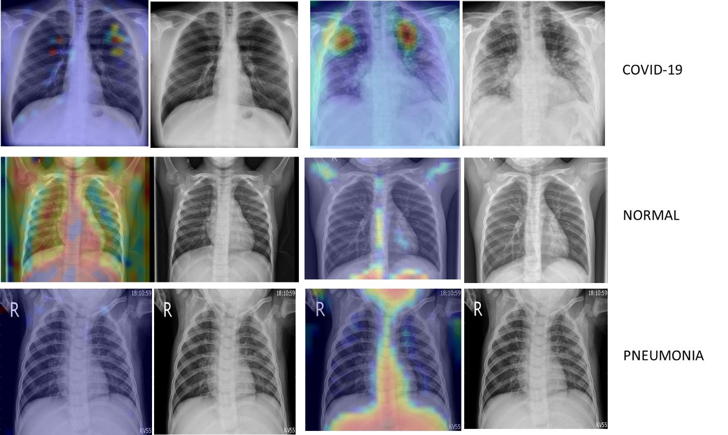
Figure 6 : Class Specific Heat Map using Grad-cam
Cross-validation is an important technique to assess the performance of a model. In k-fold cross validation, the data is split into k folds and each fold is used as a test set by the model to make predictions.
labels = ['CV', 'N','P']
img_size = 224
def fetch_data(dir):
data = []
for label in labels:
path = os.path.join(dir, label)
class_num = labels.index(label)
for img in os.listdir(path):
try:
img_arr = cv2.imread(os.path.join(path, img))[...,::-1]
resized_arr = cv2.resize(img_arr, (img_size, img_size))
data.append([resized_arr, class_num])
except Exception as e:
print(e)
return np.array(data)
data=fetch_data("/content/drive/MyDrive/Data")
a = []
b = []
for feature, label in data:
a.append(feature)
b.append(label)
# Data Normalization
a = np.array(x) / 255
a.reshape(-1, img_size, img_size, 1)
def get_model():
model =tf.keras.models.Sequential([
tf.keras.layers.Conv2D(64,(3,3),activation='relu',input_shape=(224,224,3)),
tf.keras.layers.MaxPooling2D(2,2),
tf.keras.layers.Conv2D(64,(3,3),activation='relu'),
tf.keras.layers.MaxPooling2D(2,2),
tf.keras.layers.Conv2D(128,(3,3),activation='relu'),
tf.keras.layers.MaxPooling2D(2,2),
tf.keras.layers.Conv2D(64,(3,3),activation='relu'),
tf.keras.layers.MaxPooling2D(2,2),
tf.keras.layers.Flatten(),
tf.keras.layers.Dropout(0.5),
tf.keras.layers.Dense(512,activation='relu'),
tf.keras.layers.Dense(3,activation='softmax')
])
model.compile(loss='categorical_crossentropy',optimizer='adam',metrics=['accuracy'])
return(model)
Classifier= KerasClassifier(build_fn=get_model, epochs=10, batch_size=10, verbose=0)
kfold= KFold(n_splits=6)
precision= cross_val_score(Classifier, a, b, scoring='precision_micro',cv=kfold)
print('Precision is:',precision)
accuracy= cross_val_score(Classifier, a, b, scoring='accuracy',cv=kfold)
print('Accuracy is:',accuracy)
recall= cross_val_score(Classifier, a, b, scoring='recall_micro',cv=kfold)
print('Recall is:',recall)
f1= cross_val_score(estimator, x, y, scoring='f1_micro',cv=kfold)
print('F1 score is:',f1)
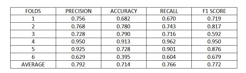
Figure 7 : K fold cross validation metrics
Using 6 folds cross validation, the model achieved 79% precision, 71% accuracy, 76% recall and 77% score, on average over different folds.
In conclusion, the proposed model looks promising in identifying and distinguishing Covid-19 from the other two classes of healthy and pneumonia. However, the major limitation of the study is the limited sample size, addressing this problem along with tuning of certain other hyper parameters can further enhance the performance of the model.
About the Author:
Write A Public Review