
Table of Contents
- What is Boosting ?
- What is Adaboost ?
- What are the Base Learners in Adaboost ?
- Where to use Adaboost ?
- Adaboost on Wine Classification Dataset.
- Conclusion
What is Boosting ?
'Boost' means to improvise anything, increase or raise performance. In terms of Datascience Boosting means to make weak learners as strong learners. Doing so helps to improve predictions and accuracy of model through sequential processing. This is an ensemble method which trains weak learners sequentially to create strong learners using the given data.
What is Adaboost ?
AdaBoost is also called as adaptive boosting. Its a sequential boosting Technique ,where weak learners are made strong learners. Here the learners are base models which can be DecisionTrees, Logistic Regression models or any other model. Adaptive boosting takes the given number of base learners, minimum of 100 and anything at the maximum. We use Adaboost Regressor for continuous response variables and Adaboost Classifier for discrete response variables.
What Are the base learners in Adaboost ?
In Adaboost, the base learners are usually DecisionTrees. You can build any amount of decision trees in Adaboost so as to solve your problem. Other base learners used include but not limited to, Logistic Regression, Random Forest, Linear Regression, Decision Trees, Support Vector Machines. Use the parameter 'base_estimator' to give the desired base learner and 'n_estimator' for the number of base estimators taken.
Where to use Adaboost ?
Adaboost works well on Binary Classification problems. Adaboost should be used in place where data is not noisy. You can use it for both classification and Regression Problems. You can use preferably more on classification problems than regression problems.
Implementation of Adaboost on Wine Data Set
    # importing and initializing Libraries
    import pandas as pd
    import matplotlib.pyplot as pl
    import seaborn as sb
    import numpy as np

    from sklearn.model_selection import train_test_split
    from sklearn.ensemble import AdaBoostClassifier
    from sklearn.metrics import accuracy_score
    from sklearn.metrics import classification_report
    from sklearn.metrics import confusion_matrix
    from sklearn.linear_model import LogisticRegression
We are going to use the wine data set for this implementation. As such multiple versions of this dataset exists on UCI, Kaggle and so on. You can infact find a small set in SkLearn also. For ease of use, we have kept a copy of the data set we have used. Click here to download the data set.
    # Importing Dataset
    wine = pd.read_csv('Z:/Imurgence/wine-data-for-adaboost.csv')

    wine
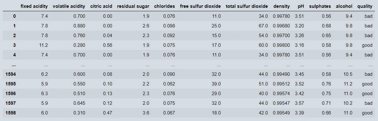 Figure 1 : Wine data set snapshot view
    # Shape of the data with number of rows and number of columns respectively
    wine.shape
(1599, 12)
    # Column Names in Dataset
    wine.columns
Index(['fixed acidity', 'volatile acidity', 'citric acid', 'residual sugar',
       'chlorides', 'free sulfur dioxide', 'total sulfur dioxide', 'density',
       'pH', 'sulphates', 'alcohol', 'quality'],
      dtype='object')
    # Number of missing values in Dataset for each variable
    wine.isna().sum()
fixed acidity           0
volatile acidity        0
citric acid             0
residual sugar          0
chlorides               0
free sulfur dioxide     0
total sulfur dioxide    0
density                 0
pH                      0
sulphates               0
alcohol                 0
quality                 0
dtype: int64
    # Finding Correlation and Multicollinearity
    # Boosting algorithms are not affected by Multicollinearity. This data has multicollinearity and we wont be taking it to consideration since we are using boosting technique.
    sb.heatmap(wine.corr())
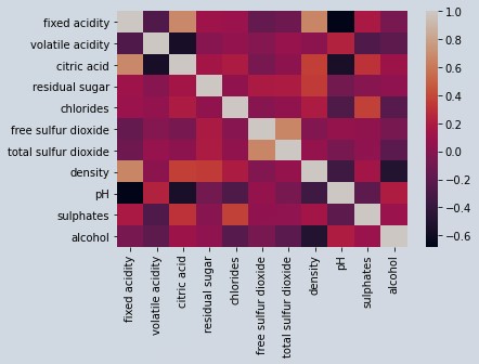 Figure 2 : Correlation grid rot wine data
    # Adaboost Classifier is affected by outliers and Noisy data.
    # Outliers are very bad for prediction using Adaboost algorithm, hence we are going to find and remove outliers if any .   # Before that we are going to split the data into features and target

    X = wine.iloc[:,0:11]     #Features
    Y = wine.iloc[:,11]       #Target

    # We are creating a grid of 3 rows x 4 colums to plot the boxplots of features
    # This would help us eyeball an check presence of Outliers

    i = 1   #initialized a counter to incrementally increase the quadrant location for plotting
    plot = pl.figure()   #create a empty plot object
    plot.subplots_adjust(hspace=1, wspace=0.2)   #define the margins between plot quadrants horizontally and vertically
    for col in X.columns:     #for loop to define quadrant, and plot individual charts
        i=i+1
        quadrant = plot.add_subplot(4, 4, i)
        sb.boxplot(X[col],ax=quadrant)
    pl.show()
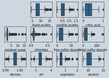 Figure 3 : Boxplot of features in wine data to check outlier presence
    # As we can see all the features have outliers, so we need to cap it
    # We are going to run it in a loop to cap the outliers at 5th and 90th percentile
    for col in X.columns:
        percentiles = X[col].quantile([0.05,0.90]).values
        X[col] = np.clip(X[col], percentiles[0], percentiles[1])

    # Redoing the same plot as in figure 3 by running the code patch on transformed data
    i = 1
    plot = pl.figure()
    plot.subplots_adjust(hspace=1, wspace=0.2)
    for col in X.columns:
        i=i+1
        quadrant = plot.add_subplot(4, 4, i)
        sb.boxplot(X[col],ax=quadrant)
    pl.show()
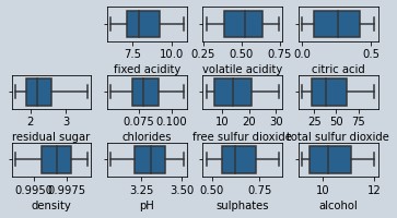 Figure 4 : Boxplot of features in wine data after removing outlier's
    # Splitting train and test data with 30 % of the data in test
    xtrain,xtest,ytrain,ytest=train_test_split(X,Y,test_size=0.3,random_state=1,stratify=Y)

    # We are using a Logistic function in adaboost, you can use the default which is decision tree
    # With decision tree, the training model can have 100?curacy but validation might have drastic drop because of overfit
    lr = LogisticRegression()
    ada_model = AdaBoostClassifier(n_estimators=600,base_estimator=lr, random_state=0)
    ada_model.fit(xtrain,ytrain)

    # predicting the target variables in training environment
    predict_train = ada_model.predict(xtrain)

    # Check the accuracy score for train data
    accuracy_score(predict_train,ytrain)

    # Publish the classification report in training environment
    print(classification_report(predict_train,ytrain))

              precision    recall  f1-score   support
         bad       0.76      0.72      0.74       545
        good       0.75      0.78      0.76       574

    accuracy                           0.75      1119
   macro avg       0.75      0.75      0.75      1119
weighted avg       0.75      0.75      0.75      1119

    # predicting the target variables in testing environment
    predict_test = ada_model.predict(xtest)

    # Check the accuracy score for test data
    accuracy_score(predict_test,ytest)

              precision    recall  f1-score   support
         bad       0.71      0.70      0.71       227
        good       0.74      0.75      0.74       253

    accuracy                           0.73       480
   macro avg       0.72      0.72      0.72       480
weighted avg       0.72      0.72      0.72       480

    # Prepare the Confusion matrix
    confusion_matrix(predict_test,ytest)
Conclusion
Adaboost is a good algorithm to ignore and still live with multicollinearity. The only problem is outliers which can be handled by capping at a specified threshold as we have demonstrated. If you want to get a good read on basic decision trees before getting into ensemble models like adaboost here is a good article on Decision Tree's in a Nutshell.
About the Author's:
Write A Public Review