
Table of Content
- Introduction
- Working of Support Vector Machine
- Support Vector Machines Kernels
- Advantages
- Disadvantages
- Support Vector Machine Use Cases
- Implementation
- Conclusion and Summary
Introduction
Support Vector Machine or SVM as it is briefly known was first introduced in the 1960's and with couple of iteration's later improvised in the 1990's. An SVM is a supervised machine learning algorithm used exclusively for classification or prediction. But the best used cases have been for classification rather than point predictions. There has been an increased adaption and popularization of this technique because of the ease of usage and high efficiency. SVM as compared to other machine learning algorithms possesses the capability of performing classification, regression, and outlier detection as well. A support vector machine is a discriminative classifier that is formally designed by a separate hyper-plane. The algorithm finds a linear hyperplane that separates the two classes using the maximum distance between the hyperplane and the nearest instance in each class.. In addition, an SVM can also perform non – linear classification. A support vector machine is a machine learning algorithm used for classification and regression. When we say its a supervised learning algorithm, we mean it learns from a series of examples with known labels, and then assigns labels to new data points.
Working of Support Vector Machine
The main objective of the Support Vector Machine is to segregate the given data in the best possible way. When the segregation is done, the distance between the nearest points is known as margin. The approach is to find a hyper-plane so as tp create the maximum possible margin between the support vectors in the given dataset. The support vector machine follows the following:
- It generates a hyper-plane that segregates the classes in the best possible ways.
- It selects the right hyper-plane with the maximum segregation from either nearest data points.
In some cases, while dealing with inseparable and non-linear plains the hyper-planes cannot be very efficient and in those cases, the SVM uses a kernel trick to transform the input into a higher dimensional space so with this it becomes easier to segregate the points.
Support Vector Machines Kernels
An SVM kernel is used to add more dimensions to a lower dimension space to make it easier to segregate the data. It converts the inseparable problems to a separable problem by adding more dimensions using the kernel trick. A Support Vector Machine is always implemented in practice by a kernel, the kernel trick helps to make it a more accurate classifier.
Different Types of the kernel in SVM are:
- Linear Kernels
- Polynomial Kernels
- Radial Basis Function Kernels
Linear Kernels
A linear kernel can be used as a normal dot product between any two given observations, the product between the vectors is the sum of the multiplication of each pair of input values.
Polynomial Kernels
A polynomial Kernel is a rather generalized form of the linear kernel, it can distinguish between curved and non-linear input phases.
Radial Basis Function Kernels (RBF)
The radial basis kernel of the RBF kernel is commonly used in SVM classification, it can map the space into infinite dimensions which is an advantage of the RBF kernel.
Advantages of SVM
- It is effective in high dimensional spaces
- It is still effective in cases where the no. of dimensions is greater than the no. of samples
- It uses a subset of training point in the decision function that makes it memory efficient
- Different kernel function can be specified for the decision function which also makes it versatile
Disadvantages of SVM
-
We may have a over fitting issue if the number of features or columns are larger that the samples or records.
-
Support Vector Machines do not directly provide probability estimate these are calculated using 5 fold cross-validation
Support Vector Machine Use Cases
- Face Detection
- Text and Hypertext Categorization
- Classification of Images
- Bioinformatics
- Remote Homology Detection
- Handwriting Detection
- Generalized Predictive Control
Implementation
Importing Libraries and Data
    import numpy as np
    import pandas as pd
    import matplotlib.pyplot as plt
    import seaborn as sns
    from sklearn.preprocessing import MinMaxScaler
    from sklearn.model_selection import train_test_split
    from sklearn.svm import SVR

    # Download the data set used in this SVM case study by clicking here
    house_df = pd.read_csv('house_sales_data.csv')

    pd.set_option('display.max_columns', None)
    house_df
               id             date     price  bedrooms       bathrooms  sqft_living  sqft_lot  floors      waterfront  view  condition  grade      sqft_above  sqft_basement  yr_built  yr_renovated      zipcode      lat     long  sqft_living15      sqft_lot15
0      7129300520  20141013T000000  221900.0         3            1.00         1180      5650     1.0               0     0          3      7            1180              0      1955             0        98178  47.5112 -122.257           1340            5650
1      6414100192  20141209T000000  538000.0         3            2.25         2570      7242     2.0               0     0          3      7            2170            400      1951          1991        98125  47.7210 -122.319           1690            7639
2      5631500400  20150225T000000  180000.0         2            1.00          770     10000     1.0               0     0          3      6             770              0      1933             0        98028  47.7379 -122.233           2720            8062
3      2487200875  20141209T000000  604000.0         4            3.00         1960      5000     1.0               0     0          5      7            1050            910      1965             0        98136  47.5208 -122.393           1360            5000
4      1954400510  20150218T000000  510000.0         3            2.00         1680      8080     1.0               0     0          3      8            1680              0      1987             0        98074  47.6168 -122.045           1800            7503
              ...              ...       ...       ...             ...          ...       ...     ...             ...   ...        ...    ...             ...            ...       ...           ...          ...      ...      ...            ...             ...
21608   263000018  20140521T000000  360000.0         3            2.50         1530      1131     3.0               0     0          3      8            1530              0      2009             0        98103  47.6993 -122.346           1530            1509
21609  6600060120  20150223T000000  400000.0         4            2.50         2310      5813     2.0               0     0          3      8            2310              0      2014             0        98146  47.5107 -122.362           1830            7200
21610  1523300141  20140623T000000  402101.0         2            0.75         1020      1350     2.0               0     0          3      7            1020              0      2009             0        98144  47.5944 -122.299           1020            2007
21611   291310100  20150116T000000  400000.0         3            2.50         1600      2388     2.0               0     0          3      8            1600              0      2004             0        98027  47.5345 -122.069           1410            1287
21612  1523300157  20141015T000000  325000.0         2            0.75         1020      1076     2.0               0     0          3      7            1020              0      2008             0        98144  47.5941 -122.299           1020            1357
Understanding the Data
    house_df.isnull().sum()

id               0
date             0
price            0
bedrooms         0
bathrooms        0
sqft_living      0
sqft_lot         0
floors           0
waterfront       0
view             0
condition        0
grade            0
sqft_above       0
sqft_basement    0
yr_built         0
yr_renovated     0
zipcode          0
lat              0
long             0
sqft_living15    0
sqft_lot15       0
dtype: int64
We observe that there are no missing values in the data.
    house_df.shape

(21613, 21)
So we have 21 columns and a total of 21,613 records. Next lets check the column names for functional understanding.
    house_df.columns

Index(['id', 'date', 'price', 'bedrooms', 'bathrooms', 'sqft_living',
       'sqft_lot', 'floors', 'waterfront', 'view', 'condition', 'grade',
       'sqft_above', 'sqft_basement', 'yr_built', 'yr_renovated', 'zipcode',
       'lat', 'long', 'sqft_living15', 'sqft_lot15'],
      dtype='object')
We need to check the summary statistics of the data. We use the describe function to understand the distribution of data
    house_df.describe()
                 id         price  ...  sqft_living15     sqft_lot15
count  2.161300e+04  2.161300e+04  ...   21613.000000   21613.000000
mean   4.580302e+09  5.400881e+05  ...    1986.552492   12768.455652
std    2.876566e+09  3.671272e+05  ...     685.391304   27304.179631
min    1.000102e+06  7.500000e+04  ...     399.000000     651.000000
25%    2.123049e+09  3.219500e+05  ...    1490.000000    5100.000000
50%    3.904930e+09  4.500000e+05  ...    1840.000000    7620.000000
75%    7.308900e+09  6.450000e+05  ...    2360.000000   10083.000000
max    9.900000e+09  7.700000e+06  ...    6210.000000  871200.000000
A quick look at the data type.
    house_df.info()

RangeIndex: 21613 entries, 0 to 21612
Data columns (total 21 columns):
 #   Column         Non-Null Count  Dtype
---  ------         --------------  -----
 0   id             21613 non-null  int64
 1   date           21613 non-null  object
 2   price          21613 non-null  float64
 3   bedrooms       21613 non-null  int64
 4   bathrooms      21613 non-null  float64
 5   sqft_living    21613 non-null  int64
 6   sqft_lot       21613 non-null  int64
 7   floors         21613 non-null  float64
 8   waterfront     21613 non-null  int64
 9   view           21613 non-null  int64
 10  condition      21613 non-null  int64
 11  grade          21613 non-null  int64
 12  sqft_above     21613 non-null  int64
 13  sqft_basement  21613 non-null  int64
 14  yr_built       21613 non-null  int64
 15  yr_renovated   21613 non-null  int64
 16  zipcode        21613 non-null  int64
 17  lat            21613 non-null  float64
 18  long           21613 non-null  float64
 19  sqft_living15  21613 non-null  int64
 20  sqft_lot15     21613 non-null  int64
dtypes: float64(5), int64(15), object(1)
memory usage: 3.5+ MB
Data Pre-Processing
    # dropping the date and id field as not required
    house_df.drop(['date', 'id'], axis = 1, inplace = True)

    plt.figure(figsize = (15,12))
    sns.heatmap(house_df.corr(), annot = True, cmap = 'magma')
    plt.show()
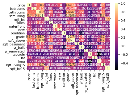
Figure 1 : House price data correlation plot
    # dropping columns which dont have corelation an relevancy
    house_df = house_df.drop(['condition', 'zipcode', 'long', 'sqft_lot15', 'waterfront', 'view', 'sqft_basement',
                             'yr_renovated'], axis = 1)
    house_df
          price  bedrooms  bathrooms  ...  yr_built      lat  sqft_living15
0      221900.0         3       1.00  ...      1955  47.5112           1340
1      538000.0         3       2.25  ...      1951  47.7210           1690
2      180000.0         2       1.00  ...      1933  47.7379           2720
3      604000.0         4       3.00  ...      1965  47.5208           1360
4      510000.0         3       2.00  ...      1987  47.6168           1800
            ...       ...        ...  ...       ...      ...            ...
21608  360000.0         3       2.50  ...      2009  47.6993           1530
21609  400000.0         4       2.50  ...      2014  47.5107           1830
21610  402101.0         2       0.75  ...      2009  47.5944           1020
21611  400000.0         3       2.50  ...      2004  47.5345           1410
21612  325000.0         2       0.75  ...      2008  47.5941           1020

[21613 rows x 11 columns]
Splitting data
    X = house_df.drop(['price'], axis = 1)
    Y = house_df['price']
Training Model
    scaler = MinMaxScaler(feature_range=(0, 1))
    scaler.fit(X)
    X_Scaler = scaler.transform(X)

    X_train, X_test, Y_train, Y_test = train_test_split(X_Scaler, Y, test_size = 0.2, random_state = 2)

    model = SVR(kernel = 'linear')
    model.fit(X_train, Y_train)
Model Evaluation
    model.score(X_test, Y_test)

    predictions = model.predict(X_test)
    predictions

array([450367.72306356, 450524.68977382, 450087.47563024, ...,
       450193.8994151 , 449453.92018701, 449700.14385532])
Prediction Using New Manual fed Data
    X_new = [[2, 0.75, 1020, 1350, 2.0, 7, 1020, 2009, 47.5944, 1020]]
    X_newScaler = scaler.transform(X_new)

    float(model.predict(X_newScaler))

450128.90560640447
Conclusion and Summary
In this tutorial, we discussed the Support Vector Machine (SVM) and using it for regression. Also, we discussed the working of a support machine, various kernels, advantages, disadvantages, and various use cases of an SVM , further on, we also built a model for predicting the house prices using various independent variables. You can check out this quick implementation of Support Vector Machines for Hand Written Alphabet Recognition.
About the Author's:
Write A Public Review