
Table of Contents
- Introduction
- Sigmoid and Logit Function
- Advantage and Disadvantage of Logistic Regression
- Importing Important Libraries and Dataset
- Data Visualization
- Splitting of Dataset to test and train
- Building model and Tuning Hyper-parameters
- Fitting the model
- Predictions using the model
- Confusion Matrix
- Classification Report
- Conclusion and Summary
Introduction
Logistic Regression is a Supervised Machine Learning Algorithm that is used for the classification of data. There can be two types of classifications using logistic regression i.e. Binary Classification and Multiclass Classification.
In Binary Classification the predicted output has 2 outcomes that can be either true (1) or false (0). So unlike the graph of linear regression, logistic regression doesn't have a straight line. It has a curved line formed using the sigmoid or logit function.
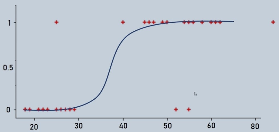
Figure 1 : Logistic Regression Curve illustration
In Multiclass Classification, the predicted output can have multiple outputs like classification of digits from 1 to 10. In these types of problems, it uses the one vs. rest approach where one is the desired output and the rest is remaining outputs.
Sigmoid and Logit Function
Sigmoid Function as represented as
F (z) = 1/1-e^ (-z)
Where Z = W0 + W1X1 + W2X2 +………+ WnXn
Logit Function
Log (P/1-P) = B0 + B1x
Advantage and Disadvantage of Logistic Regression
The advantage of using Logistic Regression is we have no issue of defining learning rate (alpha) and tuning it as a hyper-parameter. It often runs faster most of the time than other algorithms.
The major Disadvantage of using Logistic Regression is that it is more complex than other algorithms until we learn the underlying concept and basics of Logistic Regression otherwise it is a black box.
Importing Important Libraries and Dataset
    import pandas as pd
    import numpy as np
    import matplotlib.pyplot as plt
    import seaborn as sns
    import cv2
    from sklearn.datasets import fetch_openml
    from sklearn.model_selection import train_test_split
    from sklearn.linear_model import LogisticRegression
    from sklearn.metrics import confusion_matrix, classification_report

    # we need an active internet connection as we are pulling the data from openml site
    mnist = fetch_openml('mnist_784')
    mnist

    mnist.data
    mnist.data[0]
Data Visualization
    mnist.data.shape
(70000, 784)

    mnist.target

    mnist.target = [int(i) for i in mnist.target]
    mnist.target[0:10]
[5, 0, 4, 1, 9, 2, 1, 3, 1, 4]

    # check 3rd element in sample data
    plt.imshow(np.reshape(mnist.data[2], (28, 28)), cmap = 'gray')
    plt.title("Label %i" %mnist.target[2])
    plt.show()
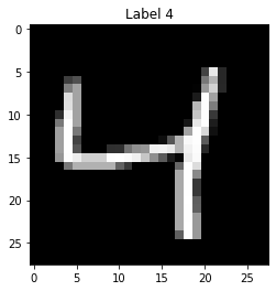
Figure 2 : Sample Image data of Digits
Splitting of Dataset to test and train
    np.reshape(mnist.data[1], (28,28))

    X = mnist.data
    Y = mnist.target

    X_train, X_test, Y_train, Y_test = train_test_split(X, Y, test_size = 0.15, random_state = 0 )
Building model and Tuning Hyper-parameters
    # Parameters for multi-class classification
    logit_model = LogisticRegression(multi_class = 'multinomial', max_iter = 1e3, C = 1, solver = 'sag')
Fitting the model
    logit_model.fit(X_train, Y_train)
    logit_model.score(X_test, Y_test)
Predictions using the model
    yhat = logit_model.predict(X_test)
    yhat
Manual Check of some sample predictions at 1st, 9th and 99th element position
    yhat[0]
0
    plt.imshow(np.reshape(X_test[0],(28,28)),cmap='gray')
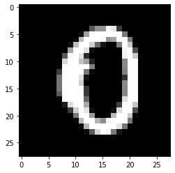
Figure 4 : First element in Predicted data set
    yhat[8]
8
    plt.imshow(np.reshape(X_test[8],(28,28)),cmap='gray')
Figure 5 : Ninth element in Predicted data set
    yhat[98]
7
    plt.imshow(np.reshape(X_test[98],(28,28)),cmap='gray')
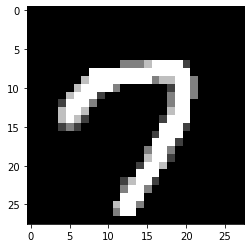
Figure 6 : Ninety ninth element in Predicted data set
Confusion Matrix
    confusion_matrix(Y_test, yhat)

array([[1019,    0,    1,    1,    3,    8,   12,    1,    6,    1],
       [   0, 1156,    7,    4,    1,    5,    2,    3,   12,    2],
       [   9,   16,  968,   22,   14,    4,   16,    9,   31,    3],
       [   4,    4,   38,  925,    1,   29,    1,   10,   25,   15],
       [   4,    3,    5,    2,  923,    1,   11,   11,    8,   35],
       [  13,    2,    9,   30,   10,  791,   21,    4,   32,   12],
       [  13,    3,    8,    0,    9,   16,  988,    2,    3,    1],
       [   4,    5,   16,    6,   12,    3,    1, 1023,    6,   44],
       [   5,   17,   10,   24,    6,   25,   10,    3,  895,   15],
       [   4,    5,    5,   13,   32,    7,    1,   36,    9,  900]],
      dtype=int64)
    plt.figure(figsize = (5, 5))
    sns.heatmap(confusion_matrix(Y_test, yhat), annot = True)
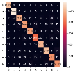
Figure 7 : Confusion Matrix for the Digit Recognition Predicted cases
Classification Report
    print(classification_report(Y_test, yhat))

              precision    recall  f1-score   support

           0       0.95      0.97      0.96      1052
           1       0.95      0.97      0.96      1192
           2       0.91      0.89      0.90      1092
           3       0.90      0.88      0.89      1052
           4       0.91      0.92      0.92      1003
           5       0.89      0.86      0.87       924
           6       0.93      0.95      0.94      1043
           7       0.93      0.91      0.92      1120
           8       0.87      0.89      0.88      1010
           9       0.88      0.89      0.88      1012

    accuracy                           0.91     10500
   macro avg       0.91      0.91      0.91     10500
weighted avg       0.91      0.91      0.91     10500
Conclusion and Summary
In this tutorial, we discovered how to predict digits using a multiclass classification logistic regression model in python. Also, we learned how to build, train and test models by importing the MNIST dataset.
The predictions are also made by importing the data as we an image of a digit 2 and the model predicted it correctly. The classification report and Confusion matrix displayed the strength and weaknesses of our model. Read more about hand written text recognition using Support Vector Machine.
About the Author's:
Write A Public Review