
Table of Content
- What is Artificial Neural Network?
- Example of Artificial Neural Network
- Working of an Artificial Neural Network
- Modes in Perceptron
- Different Activation Functions
- Perceptron Training with Analogy
- Multilayer Perceptron of Artificial Neural Network
- Training an Artificial Neural Network
- Application of Artificial Neural Network
- Implementation
- Conclusion and Summary
What is Artificial Neural Network?
Artificial Neural Network (ANN) is a computing system that is designed to simulate the way the human brain analysis and processes information. Artificial Neural Network has self-learning capabilities that enable's it to produce better results as more data become available. So if you train your network on more data it will be more accurate. So this neural network learns by examples and you can configure your neural network for the specific application. It can be pattern recognition, data classification anything else. Because of neural network we see a lot of new technologies have evolved from translating web pages to other languages, to having virtual assistants to order groceries online, to conversing with chat bots, neural networks have made these possible. In a nutshell, an artificial neural network is a network of various artificial neurons.
Example of Artificial Neural Network
Let us consider two scenarios before and after artificial neural networks. So we have a machine and we have trained this machine with images of four types of dogs. Once the training is done, we provide a random image to this machine which has a dog but this dog is not like the other dogs on which we have trained the model. So ideally, it should not be able to recognize it as a dog.
Without the ANN model, our machine cannot identify the dog in the picture. But how does it do this. Well, our machine will be confused and it cannot figure out where the dog is but when we talk about neural networks, even if we have not trained our machine on this specific dog, but still it can identify a certain feature of the dog that we have trained on like four legs, one tail and so on. It can match those features with the dog that is there in the particular testing image and it can identify that as dog. This happens all because of artificial neural networks.
Working of an Artificial Neural Network
So here let's begin by explaining a single artificial neuron that is called Perceptron.
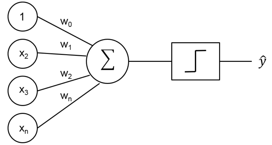
Figure 1 : Perceptron Schematic Diagram
As shown in Figure 1, over the left side, we have multiple inputs X1, X2, ….. Xn and we have corresponding weights as well W1 for X1, W2 for X2, ….. Wn for Xn. Then we calculate the weighted sum of these inputs and after doing that we pass it through an activation function. This activation function provides a threshold value such that, above that value neuron will fire else it won't fire so. An artificial neural network involves a lot of these artificial neurons with their activation function and their elements.
Modes in Perceptron
There are two modes in perceptron –
- Training Mode
- Using Mode
Training Mode
In training mode, the neuron can be trained to fire for particular input patterns which means that we will train our neurons to fire on a certain set of inputs and to not fire on another set of inputs.
Using Mode
It means that when we our input pattern is detected at the input, its associated output becomes the current output. This means that once the training is done and we provide an input on which the neuron has been trained, it will detect the input and will provide the associated output.
Different Activation Functions
Some major activation functions are –
- Step Function
- Sigmoid Function
- Sign Function
Step Function
In step function the moment our input is greater than a particular value our neuron will fire else it won’t.
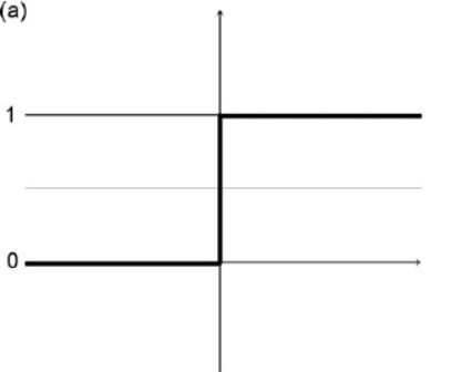
Figure 2 : Step Function Schematic Diagram
Sigmoid Function
A sigmoid function maps the entire number range into a small range such as between 0 and 1, so one use of the sigmoid function is to convert a real value into one that can be interpreted as a probability.
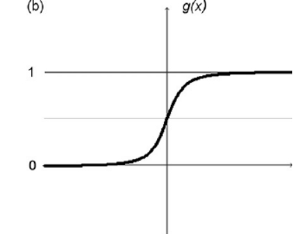
Figure 3 : Sigmoid Function Schematic Diagram
Sign Function
A sign function as called a signum function, is -1 for all negative numbers, 0 for the number 0, and 1 for all positive numbers.
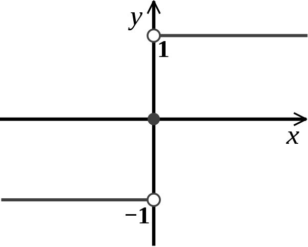
Figure 4 : Sign Function Schematic Diagram
Perceptron Training with Analogy – Cricket Analogy
There is a cricket match happening near your house and you want to badly go there but your decision depends on three factors –
- How is the weather, is it good or bad
- Your friend is going with you or not
- Any public transport is available
So on these factors, your decision will depend on whether you will go or not. We will consider these factors as input to our perceptron and will consider a decision of going or not going to the cricket match.
Let us consider the state of weather as X1, so when the weather is good it will be 1 and we will go and when the weather is bad it will be 0 and we will not go. Similarly, your friend is going with you or not that will be X2 and if he/she is going it will be 1, and if not it will be 0. Similarly for public transport if it is available then it is 1 else it is 0. These are three inputs now let us consider the output it will be 1 when you are going and 0 when you are not going.
But we will not give importance to each factor equally i.e. certain factors are of high priority for us and we will focus on these factors more whereas some factors won't affect us that much.
Here the most important factor is the weather. So if the weather is good we don't care that friend is going with me or not or if there is public transport available or not. It means when X1 is high, output will be high so we will use weights to priorities our factors. We assign high weights to more important factors or more important inputs and we assign low weights to those particular inputs which are not that important to us.
So let’s assign weights –
W1 = W1 is associated with X1 = 6
W2 = W2 is associated with X2 = 2
W3 = W3 is associated with X3 = 2
We assign a pretty high weight to weather as it is an important factor and W2 and W3 are not that much important.
Threshold = 5
Threshold value means that when the weighted sum of other input is greater than 5 then only our neurons will fire or we can say then only you can go to the cricket match.
Testcase –
So when weather is good and friend is not willing to go also there is no public transport available
= 1*6 + 0*2 + 0*2
= 6
=6 > 5(Threshold)
That means our output will be 1 or we can say that we will go for the cricket match.
Multilayer Perceptron of Artificial Neural Network
This is how an artificial neural network looks like –
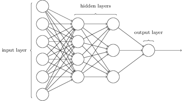
Figure 5 : Artificial Neural Network Schematic Diagram
Over here we have multiple neurons present in different layers, the 1st layer is always your input layer this is where you feed your input, then we have 1st hidden layer, then we have 2nd hidden layer, and then we have output layer although the numbers of hidden layers depend on your application or what are you working on. The problems complexity determines how many hidden layers we will have.
So we provide some input to our 1st layer and after some function, the output of these neurons become input to the next layer which is hidden layer 1.Then these layers will have various neurons, these neurons will have different activation functions so they will perform their function on the input that has been received from the previous layer and then the output of this layer will be the input to the next hidden layer 2, similarly output to hidden layer 2 will be input to the output layer and finally we get the output.
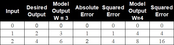
Training an Artificial Neural Network
The most common deep learning algorithm for supervised learning of multilayer perceptron is known as back-propagation. In back-propagation after the weighted sum of inputs is passing through the activation function we propagate backward and update the weights to reduce the error (desired output model). Consider the below example.
| Input | Desired Output |
|---|---|
| 0 | 0 |
| 1 | 2 |
| 2 | 4 |
In back-propagation after the weighted sum of input is passes through an activation function the corresponding output is compared to that output of the actual output that we already know, we figure out how much is the difference and then we calculate the error and based on that error what we do is propagate backward.
Application of Artificial Neural Network
Artificial Neural Network has wide range of application in field of Medicine and Business. For instance its used in Modeling and Diagnosing the cardiovascular system as well as Marketing, credit evaluation, etc.
Implementation
Importing Libraries
    import pandas as pd
    import numpy as np
    import matplotlib.pyplot as plt
    import seaborn as sns
    from sklearn.utils import resample
    from sklearn.preprocessing import LabelEncoder
    from sklearn.model_selection import train_test_split
    from keras.layers import Dense
    from keras.models import Sequential
    from keras.optimizers import Adam
    from sklearn.metrics import confusion_matrix
    from sklearn.metrics import classification_report

    # Download Online Shoppers Intention dataset from here
    # Data donated by Department of Computer Engineering, Faculty of Engineering and Natural Sciences, Bahcesehir University, Istanbul, Turkey and maintained on UCI Machine Learning Repository
    # Read through the data dictionary to understnd the variables better
    shoppers_df = pd.read_csv('Online-Shoppers-Intention.csv')
Data Visualization
    display(shoppers_df)

       Administrative  Administrative_Duration  ...  Weekend  Revenue
0                 0.0                      0.0  ...    False    False
1                 0.0                      0.0  ...    False    False
2                 0.0                     -1.0  ...    False    False
3                 0.0                      0.0  ...    False    False
4                 0.0                      0.0  ...     True    False
                  ...                      ...  ...      ...      ...
12325             3.0                    145.0  ...     True    False
12326             0.0                      0.0  ...     True    False
12327             0.0                      0.0  ...     True    False
12328             4.0                     75.0  ...    False    False
12329             0.0                      0.0  ...     True    False

[12330 rows x 18 columns]
    shoppers_df.shape

(12330, 18)

    shoppers_df.isnull().sum()

Administrative             14
Administrative_Duration    14
Informational              14
Informational_Duration     14
ProductRelated             14
ProductRelated_Duration    14
BounceRates                14
ExitRates                  14
PageValues                  0
SpecialDay                  0
Month                       0
OperatingSystems            0
Browser                     0
Region                      0
TrafficType                 0
VisitorType                 0
Weekend                     0
Revenue                     0
dtype: int64
    shoppers_df['Informational'].unique()

array([ 0.,  1.,  2.,  4., 16.,  5.,  3., 14.,  6., 12.,  7., nan,  9.,
       10.,  8., 11., 24., 13.])
    shoppers_df.dropna(inplace=True)
    shoppers_df.isnull().sum()

Administrative             0
Administrative_Duration    0
Informational              0
Informational_Duration     0
ProductRelated             0
ProductRelated_Duration    0
BounceRates                0
ExitRates                  0
PageValues                 0
SpecialDay                 0
Month                      0
OperatingSystems           0
Browser                    0
Region                     0
TrafficType                0
VisitorType                0
Weekend                    0
Revenue                    0
dtype: int64
Exploratory Data Analysis
sns.catplot(x = 'Revenue', kind = 'count', data = shoppers_df)
plt.show()
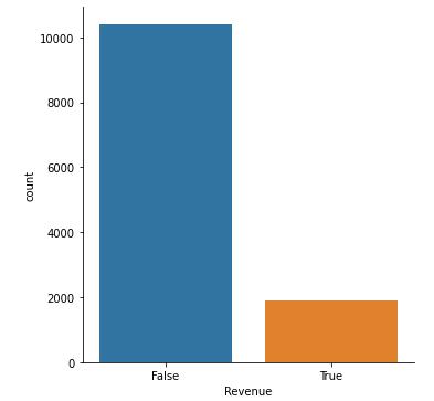 Figure 6 : Plot Count of Revenue Flags
sns.catplot(x = 'Weekend', kind = 'count', data = shoppers_df, palette='magma')
plt.show()
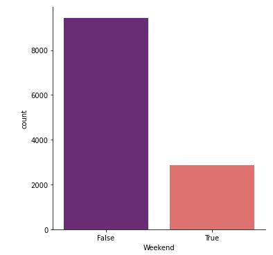 Figure 7 : Plot Count of Weekend Flags
shoppers_df['VisitorType'].value_counts()
plt.figure(figsize=(10,10))
data = [10537, 1694, 85]
colors = ['darkviolet', 'violet', 'pink']
label = ['Returning_Visitor', 'New_Visitor', 'Other']
plt.pie(data, colors = colors, labels = label, autopct='%0.2f%%')
plt.show()
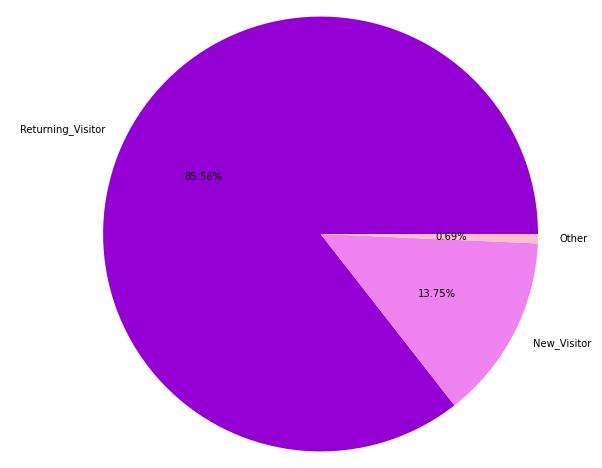 Figure 8 : Plot of proportion of Customers basis Return Type
plt.figure(figsize=(12,8))
sns.catplot(x = 'Revenue', kind = 'count', hue = 'VisitorType', data = shoppers_df, palette = 'magma')
plt.show()
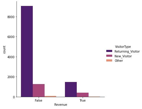 Figure 9 : Plot of Return Type of Shopper's basis Return Type
sns.catplot(x = 'Region', kind = 'count', data = shoppers_df, height=8, palette= 'RdYlGn')
plt.show()
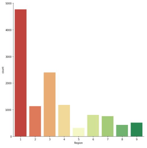 Figure 10 : Plot of Shopper's by Region
sns.catplot(x = 'Region', kind = 'count', data = shoppers_df[shoppers_df['Revenue'] == True], height=8, palette= 'magma')
plt.show()
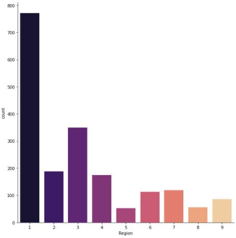 Figure 11 : Plot of Shopper's by Region given revenue is Flagged True
Data Augmentation
    shoppers_df['Revenue'].value_counts()

False    10408
True      1908
Name: Revenue, dtype: int64
df_0 = shoppers_df[shoppers_df['Revenue'] == False]
df_1 = shoppers_df[shoppers_df['Revenue'] == True]
df_1_upsample = resample(df_1, n_samples = 8000, replace = True, random_state = 123)
shoppers_df2 = pd.concat([df_0, df_1_upsample])
sns.catplot(x = 'Revenue', kind = 'count', data = shoppers_df2.drop_duplicates())
plt.show()
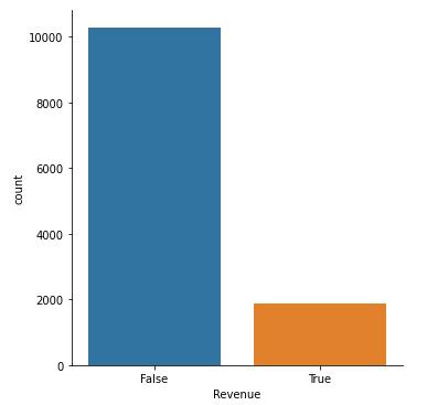 Figure 12 : Plot of Revenue without Duplicate Shoppers
sns.catplot(x = 'Revenue', kind = 'count', data = shoppers_df2)
plt.show()
Figure 12 : Plot of Revenue without Duplicate Shoppers
sns.catplot(x = 'Revenue', kind = 'count', data = shoppers_df2)
plt.show()
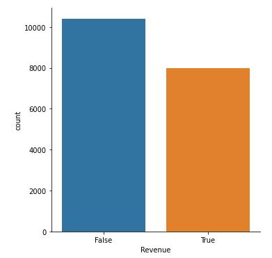 Figure 13 : Plot of Revenue with Duplicate Shoppers
shoppers_df2['Revenue'].value_counts()
False 10408
True 8000
Name: Revenue, dtype: int64
Figure 13 : Plot of Revenue with Duplicate Shoppers
shoppers_df2['Revenue'].value_counts()
False 10408
True 8000
Name: Revenue, dtype: int64
Data Preprocessing
    le = LabelEncoder()
    le.fit(shoppers_df2['VisitorType'].drop_duplicates())

    shoppers_df2['VisitorType'] = le.transform(shoppers_df2['VisitorType'])
    le.fit(shoppers_df2['Month'].drop_duplicates())

    shoppers_df2['Month'] = le.transform(shoppers_df2['Month'])
Feature Selection
    X = shoppers_df2.drop(['ProductRelated', 'BounceRates', 'Revenue'], axis = 1)
    Y = shoppers_df2['Revenue']
    X.info()


Int64Index: 18408 entries, 0 to 5986
Data columns (total 15 columns):
 #   Column                   Non-Null Count  Dtype
---  ------                   --------------  -----
 0   Administrative           18408 non-null  float64
 1   Administrative_Duration  18408 non-null  float64
 2   Informational            18408 non-null  float64
 3   Informational_Duration   18408 non-null  float64
 4   ProductRelated_Duration  18408 non-null  float64
 5   ExitRates                18408 non-null  float64
 6   PageValues               18408 non-null  float64
 7   SpecialDay               18408 non-null  float64
 8   Month                    18408 non-null  int32
 9   OperatingSystems         18408 non-null  int64
 10  Browser                  18408 non-null  int64
 11  Region                   18408 non-null  int64
 12  TrafficType              18408 non-null  int64
 13  VisitorType              18408 non-null  int32
 14  Weekend                  18408 non-null  bool
dtypes: bool(1), float64(8), int32(2), int64(4)
memory usage: 2.0 MB

    le = LabelEncoder()
    X['Weekend'] = le.fit_transform(X['Weekend'])
    X

       Administrative  Administrative_Duration  ...  VisitorType  Weekend
0                 0.0                    0.000  ...            2        0
1                 0.0                    0.000  ...            2        0
2                 0.0                   -1.000  ...            2        0
3                 0.0                    0.000  ...            2        0
4                 0.0                    0.000  ...            2        1
                  ...                      ...  ...          ...      ...
7556              8.0                  203.600  ...            2        0
7084              0.0                    0.000  ...            2        1
11927             4.0                  140.675  ...            2        1
11083             1.0                   11.000  ...            2        1
5986              3.0                   29.200  ...            2        0

[18408 rows x 15 columns]
Train Test Split
X_train, X_test, Y_train, Y_test = train_test_split(X, Y, test_size = 0.2, random_state = 3)
Building Model
    def build_model ():
      model = Sequential()
      # Input Layer : num of neurons = (2)^n
      model.add(Dense(units = 64, activation='relu', input_shape = [len(X.keys())]))
      # Hidden Layer - I
      model.add(Dense(units = 128, activation='relu'))
      # Hidden Layer - II
      model.add(Dense(units = 256, activation='relu'))
      # Output Layer
      model.add(Dense(units = 1, activation='sigmoid'))

      # Optimizers = Adam
      # Alpha = Learning Rate : sample size = small (0.001), sample size = large (0.01)
      optimizers = Adam(learning_rate= 0.0001)

      # For binary classification
      # if activation is sigmoid and o/p is binary : loss = 'binary_crossentropy'
      # if activation is softmax and o/p is binary : loss = 'categorical_crossentropy'
      model.compile(loss = 'binary_crossentropy', optimizer = optimizers, metrics = ['accuracy'])

      return model

    # Use the User defined Function to build the architecture of your model
    model = build_model()
Model Summary
    model.summary()

Model: "sequential"
_________________________________________________________________
Layer (type)                 Output Shape              Param #
=================================================================
dense (Dense)                (None, 64)                1024
_________________________________________________________________
dense_1 (Dense)              (None, 128)               8320
_________________________________________________________________
dense_2 (Dense)              (None, 256)               33024
_________________________________________________________________
dense_3 (Dense)              (None, 1)                 257
=================================================================
Total params: 42,625
Trainable params: 42,625
Non-trainable params: 0
Training Model
    results = model.fit(X_train, Y_train, epochs = 600, batch_size = 25, validation_split = 0.20)

Epoch 1/600
472/472 [==============================] - 5s 5ms/step - loss: 1.7869 - accuracy: 0.6381 - val_loss: 1.4107 - val_accuracy: 0.6446
Epoch 2/600
472/472 [==============================] - 1s 2ms/step - loss: 1.4154 - accuracy: 0.7128 - val_loss: 0.8804 - val_accuracy: 0.7468
Epoch 3/600
472/472 [==============================] - 1s 2ms/step - loss: 0.9582 - accuracy: 0.7501 - val_loss: 0.8899 - val_accuracy: 0.7461
Epoch 4/600
472/472 [==============================] - 1s 2ms/step - loss: 1.5424 - accuracy: 0.7386 - val_loss: 0.5371 - val_accuracy: 0.8075
Epoch 5/600
472/472 [==============================] - 1s 2ms/step - loss: 0.9904 - accuracy: 0.7511 - val_loss: 0.6947 - val_accuracy: 0.7777
.
.
.
.
.
Epoch 595/600
472/472 [==============================] - 1s 2ms/step - loss: 0.1871 - accuracy: 0.9154 - val_loss: 0.5160 - val_accuracy: 0.8819
Epoch 596/600
472/472 [==============================] - 1s 2ms/step - loss: 0.1952 - accuracy: 0.9163 - val_loss: 0.4959 - val_accuracy: 0.8775
Epoch 597/600
472/472 [==============================] - 1s 2ms/step - loss: 0.1866 - accuracy: 0.9172 - val_loss: 0.5104 - val_accuracy: 0.8730
Epoch 598/600
472/472 [==============================] - 1s 2ms/step - loss: 0.1860 - accuracy: 0.9166 - val_loss: 0.4913 - val_accuracy: 0.8849
Epoch 599/600
472/472 [==============================] - 1s 2ms/step - loss: 0.1827 - accuracy: 0.9207 - val_loss: 0.4855 - val_accuracy: 0.8832
Epoch 600/600
472/472 [==============================] - 1s 2ms/step - loss: 0.1825 - accuracy: 0.9194 - val_loss: 0.5192 - val_accuracy: 0.8785
Model Evaluation
    pd.DataFrame(results.history)

         loss  accuracy  val_loss  val_accuracy
0    0.571641  0.809847  0.514936      0.801426
1    0.614798  0.797538  0.416106      0.841480
2    0.568984  0.812394  1.600190      0.701629
3    0.591839  0.809423  0.454467      0.832315
4    0.545954  0.815365  0.507862      0.802783
..        ...       ...       ...           ...
595  0.195228  0.916299  0.495907      0.877461
596  0.186634  0.917233  0.510386      0.873048
597  0.186005  0.916638  0.491259      0.884929
598  0.182690  0.920713  0.485488      0.883232
599  0.182531  0.919355  0.519171      0.878479

[600 rows x 4 columns]
pd.DataFrame(results.history)[['accuracy', 'val_accuracy','loss', 'val_loss']].plot()
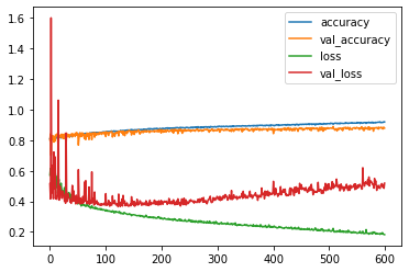
Figure 14 : Plot of Model Evaluation
    model.evaluate(X_test, Y_test)

116/116 [==============================] - 0s 991us/step - loss: 0.4559 - accuracy: 0.8851
[0.4558551609516144, 0.8851167559623718]
Predictions Using Model
    predictions = model.predict(X_test)
    yhat = np.round(predictions)

    X_New = [[0.0, 0.000, 0.0, 0.00, 0264.00000, 0.100000, 32.000000, 0.0, 2, 2, 2, 1, 2, 3, 0]]
    X_data = pd.DataFrame(X_New)
    np.round(model.predict(X_data))
Confusion Matrix
    confusion_matrix(Y_test, yhat)

array([[1751,  298],
       [ 125, 1508]], dtype=int64)

    sns.heatmap(confusion_matrix(Y_test, yhat), annot = True, fmt='0.0f')
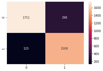
Figure 15 : Heat Map of Confusion Matrix
Classification Report
    print(classification_report(Y_test, yhat))

              precision    recall  f1-score   support

       False       0.93      0.85      0.89      2049
        True       0.83      0.92      0.88      1633

    accuracy                           0.89      3682
   macro avg       0.88      0.89      0.88      3682
weighted avg       0.89      0.89      0.89      3682
Conclusion
From this blog we understand Artificial Neural Network (ANN) a Deep Learning algorithm further on we learned about the working of an ANN model, Activation Functions, Multilayer ANN Model, and at last we also implemented the model to find about shoppers intentions. Also do read this case study on usage on CNN for Face Mask Detection which is an advance implementation of ANN
About the Author's:
Write A Public Review