
Table of Content:
- About Regularization
- Types of Penalties
- Regularization Technique
- Lasso Regression
- Example Of Lasso Regression
- Conclusion
About Regularization
To understand Lasso Regression, first we have to know what is Regularization.
So, Regularization is the concept that is used to avoid over fitting of the data by adding penalty to achieve less variance with the test data. The model is likely to perform better at prediction thereafter.
In simple term, it reduces parameters and simplifies the model so that it has the lowest over fitting or say less variance with test data, hence better prediction with test data.
For example, when we are training the model with train dataset which have two nodes, it fitted well with a straight line and for this its residual become zero. But when we test the model with test dataset we get high variance, which means our model is over fitted and we have to remove it.
It is observed that when we train our model it gives 100 percent accuracy on train data, but when we test it with test dataset its accuracy is substantially lower.
Types of Penalties
Regularization works by biasing data equal to or nearly equal to zero. In simple words it shrinks the slope of the data to find the best fit. Note the two Types of penalties as below.
L1 regularization
It adds a L1 penalty to the absolute or mode value of the magnitude of coefficient. In this process some coefficient can become zero and eliminated from model.
L2 regularization
It adds a L2 penalty to the square of the magnitude of coefficient. In this, all coefficients will shrink by the same factor to find the best fit for the model.
Regularization Technique
There are two main regularization techniques:
- Ridge Regression
- Lasso Regression.
Both have different way of assigning a penalty to the coefficients. In this article, we will learn about Lasso Regularization technique.
Lasso Regression
“LASSO” stands for Least Absolute Shrinkage and Selection Operator. This model uses shrinkage. Shrinkage basically means that the data points are recalibrated by adding a penalty so as to shrink the coefficients to zero if they are not substantial.
It uses L1 regularization penalty technique. This particular type of regression is well-suited for models showing high levels of multicollinearity or when we have to automate certain parts of model selection, like parameter elimination or feature selection.
We can represent Lasso loss functions mathematically as:
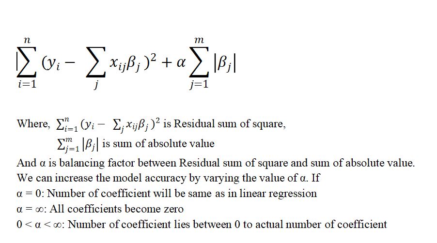
Figure 1 : Mathematical Formulation for LASSO Loss Function
Example Of Lasso Regression
    import numpy as np
    import pandas as pd
    from sklearn.model_selection import train_test_split
    from sklearn.preprocessing  import StandardScaler
    from sklearn.linear_model import Lasso
    from sklearn.metrics import r2_score as ac
Load the data set by clicking on this link - Vehicle Price dataset
    price_data = pd.read_csv('vehicle_price.csv')
    price_data.head(5)

   Unnamed: 0                              Name  ...  New_Price  Price
0           0            Maruti Wagon R LXI CNG  ...        NaN   1.75
1           1  Hyundai Creta 1.6 CRDi SX Option  ...        NaN  12.50
2           2                      Honda Jazz V  ...  8.61 Lakh   4.50
3           3                 Maruti Ertiga VDI  ...        NaN   6.00
4           4   Audi A4 New 2.0 TDI Multitronic  ...        NaN  17.74
    price_data.info()


RangeIndex: 6019 entries, 0 to 6018
Data columns (total 14 columns):
 #   Column             Non-Null Count  Dtype
---  ------             --------------  -----
 0   Unnamed: 0         6019 non-null   int64
 1   Name               6019 non-null   object
 2   Location           6019 non-null   object
 3   Year               6019 non-null   int64
 4   Kilometers_Driven  6019 non-null   int64
 5   Fuel_Type          6019 non-null   object
 6   Transmission       6019 non-null   object
 7   Owner_Type         6019 non-null   object
 8   Mileage            6017 non-null   object
 9   Engine             5983 non-null   object
 10  Power              5983 non-null   object
 11  Seats              5977 non-null   float64
 12  New_Price          824 non-null    object
 13  Price              6019 non-null   float64
dtypes: float64(2), int64(3), object(9)
memory usage: 658.5+ KB
    price_data.isnull().sum()

Unnamed: 0              0
Name                    0
Location                0
Year                    0
Kilometers_Driven       0
Fuel_Type               0
Transmission            0
Owner_Type              0
Mileage                 2
Engine                 36
Power                  36
Seats                  42
New_Price            5195
Price                   0
dtype: int64
    # Droping location, new price and unnamed column
    price_data = price_data.drop(['Unnamed: 0', 'New_Price','Location'], axis=1)
    price_data = price_data.dropna()
    price_data = price_data.reset_index(drop=True)

    price_data['Fuel_Type'].value_counts()

Diesel    3195
Petrol    2714
CNG         56
LPG         10
Name: Fuel_Type, dtype: int64

    price_data['Transmission'].value_counts()

Manual       4266
Automatic    1709
Name: Transmission, dtype: int64

    price_data['Owner_Type'].value_counts()

First             4903
Second             953
Third              111
Fourth & Above       8
Name: Owner_Type, dtype: int64
    # Lets split some columns to make a new feature
    train_df = price_data.copy()
    name = train_df['Name'].str.split(" ", n =2, expand = True)
    train_df['Company'] = name[0]
    train_df['Model'] = name[1]

    train_df['Mileage'] = train_df['Mileage'].str.split(" ", n=1, expand = True).get(0)
    train_df['Engine'] = train_df['Engine'].str.split(" ", n=1, expand = True).get(0)
    train_df['Power'] = train_df['Power'].str.split(" ", n=1, expand = True).get(0)

    train_df = train_df.drop(['Name'], axis = 1)
    train_df['Mileage'] = train_df['Mileage'].astype(float)
    train_df['Engine'] = train_df['Engine'].astype(int)
    train_df.replace("null", np.nan, inplace = True)

    train_df = train_df.dropna()
    train_df = train_df.reset_index(drop=True)
    train_df['Power'] = train_df['Power'].astype(float)

    train_df['Company'].value_counts()

Maruti           1175
Hyundai          1058
Honda             600
Toyota            394
Mercedes-Benz     316
Volkswagen        314
Ford              294
Mahindra          268
BMW               262
Audi              235
Tata              183
Skoda             172
Renault           145
Chevrolet         120
Nissan             89
Land               57
Jaguar             40
Mitsubishi         27
Mini               26
Fiat               23
Volvo              21
Porsche            16
Jeep               15
Datsun             13
Force               3
ISUZU               2
Bentley             1
Ambassador          1
Isuzu               1
Lamborghini         1
Name: Company, dtype: int64

    train_df['Company'] = train_df['Company'].replace('ISUZU', 'Isuzu')
    # Handling Rare Categorical Feature
    cat_features = [feature for feature in train_df.columns if train_df[feature].dtype == 'O']

    for feature in cat_features:
        temp = train_df.groupby(feature)['Price'].count()/len(train_df)
        temp_df = temp[temp > 0.01].index
        train_df[feature] = np.where(train_df[feature].isin(temp_df), train_df[feature], 'Rare')
    train_df['Company'].value_counts()

Maruti           1175
Hyundai          1058
Honda             600
Toyota            394
Mercedes-Benz     316
Volkswagen        314
Ford              294
Mahindra          268
BMW               262
Rare              247
Audi              235
Tata              183
Skoda             172
Renault           145
Chevrolet         120
Nissan             89
Name: Company, dtype: int64

    train_df.info()


RangeIndex: 5872 entries, 0 to 5871
Data columns (total 12 columns):
 #   Column             Non-Null Count  Dtype
---  ------             --------------  -----
 0   Year               5872 non-null   int64
 1   Kilometers_Driven  5872 non-null   int64
 2   Fuel_Type          5872 non-null   object
 3   Transmission       5872 non-null   object
 4   Owner_Type         5872 non-null   object
 5   Mileage            5872 non-null   float64
 6   Engine             5872 non-null   int32
 7   Power              5872 non-null   float64
 8   Seats              5872 non-null   float64
 9   Price              5872 non-null   float64
 10  Company            5872 non-null   object
 11  Model              5872 non-null   object
dtypes: float64(4), int32(1), int64(2), object(5)
memory usage: 527.7+ KB

    train_df['Seats'] = train_df['Seats'].astype(int)
    # Encoding Categorical data
    columns = ['Fuel_Type','Transmission','Owner_Type','Company','Model']
    def categorical_ohe(multicolumns):
        df = train_df.copy()
        i = 0
        for fields in multicolumns:
            print(fields)
            d1 = pd.get_dummies(train_df[fields])
            train_df.drop([fields], axis = 1)
            if i == 0:
                df = d1.copy()
            else:
                df = pd.concat([df, d1], axis = 1)
            i = i + 1
        df = pd.concat([df,train_df], axis = 1)
        return df

    final_df = categorical_ohe(columns)
    final_df = final_df.loc[:,~final_df.columns.duplicated()]

    now = datetime.datetime.now()
    final_df['Year'] = final_df['Year'].apply(lambda x : now.year - x)

    corr = final_df.corr()
    corr

             Diesel    Petrol      Rare  ...     Power     Seats     Price
Diesel     1.000000 -0.977947 -0.113891  ...  0.292420  0.309581  0.321035
Petrol    -0.977947  1.000000 -0.096114  ... -0.272662 -0.303177 -0.309363
Rare      -0.113891 -0.096114  1.000000  ... -0.096618 -0.033244 -0.058408
Automatic  0.139557 -0.125612 -0.067592  ...  0.644688 -0.074554  0.585623
Manual    -0.139557  0.125612  0.067592  ... -0.644688  0.074554 -0.585623
            ...       ...       ...  ...       ...       ...       ...
Mileage    0.097562 -0.130056  0.153696  ... -0.538844 -0.331576 -0.341652
Engine     0.430151 -0.410837 -0.095742  ...  0.866301  0.401116  0.658047
Power      0.292420 -0.272662 -0.096618  ...  1.000000  0.101460  0.772843
Seats      0.309581 -0.303177 -0.033244  ...  0.101460  1.000000  0.055547
Price      0.321035 -0.309363 -0.058408  ...  0.772843  0.055547  1.000000

    corr[corr['Price'] > 0.4]

             Diesel    Petrol      Rare  ...     Power     Seats     Price
Automatic  0.139557 -0.125612 -0.067592  ...  0.644688 -0.074554  0.585623
Engine     0.430151 -0.410837 -0.095742  ...  0.866301  0.401116  0.658047
Power      0.292420 -0.272662 -0.096618  ...  1.000000  0.101460  0.772843
Price      0.321035 -0.309363 -0.058408  ...  0.772843  0.055547  1.000000
    df = final_df.drop(final_df[columns],axis=1)

    X = df.drop(['Price'],axis=1)
    y = df['Price']

    X.head(5)
   Diesel  Petrol  Rare  Automatic  ...  Mileage  Engine   Power  Seats
0       0       0     1          0  ...    26.60     998   58.16      5
1       1       0     0          0  ...    19.67    1582  126.20      5
2       0       1     0          0  ...    18.20    1199   88.70      5
3       1       0     0          0  ...    20.77    1248   88.76      7
4       1       0     0          1  ...    15.20    1968  140.80      5
    # Splitting Dataset into training and testing data
    X_train, X_test, y_train, y_test = train_test_split(X, y, test_size= 0.2, random_state = 0)

    # Feature Scaling
    scaler = StandardScaler()
    scaler.fit(X)
    X_train = scaler.transform(X_train)
    X_test = scaler.transform(X_test)

    best_alpha = 0.00099
    regr = Lasso(alpha=best_alpha, max_iter=50000)
    regr.fit(X_train,y_train)

    y_pred = regr.predict(X_test)

    ac(y_test,y_pred)
0.7761524710799422
Conclusion
In this article we have learnt about Regularization, types of penalty in regularization and techniques or types of regularization. And then we have learnt about Lasso Regression in brief and how to implement it. In our model we got the accuracy of 77% which can be further increased by hyperparameter tuning, in case you don’t have any idea about how to do hyperparameter tuning you can please refer to this previous article about how to do hyperparameter tuning.
About the Author's:
Write A Public Review