
Table Of Content
- Introduction
- RFM Modeling / Analysis
- Import Dataset and Libraries
- Creating RFM Table
- Finding no. of clusters
- Conclusion
Introduction
In business it is important to know about your customers and their needs, but it is very difficult and time consuming to provide personalized service for each customer so, we group them on different characteristic and buying behavior which is known as Customer segmentation.
Grouping customers can help in understanding their behavior and also help company to do target marketing which increase the sales of company. One of the methods for customer segmentation is RFM analysis.
In this article we will learn about what RFM modeling is and how we can do this in retail sector.
RFM Modeling
In RFM modeling R stands for Recency, F stands for Frequency and M stands for Monetary. In this analysis customers grouped on the basis of their purchase history, how recently they purchased any product from company (Recency), how often they purchase (Frequency) and how much did they buy (Monetary).
We assign value of R, F and M for each customer; let’s take an example of retail product to understand it. Suppose a customer bought two products in an interval of one months of each price of 10K, here the value of R is 1 as last transaction of customer was in last month and he bought only one product in a month, value of F will be 2 as customer bought total 2 products and M will be 20K as he bought two product each of 10K.
So, till now we have assigned the value to a customers but the question is how we can find the best customer among them.
Are they from who spend the most money in your product? But what happen if they bought year ago from you and they are no longer your customer, are they still your best customers? Probably the answer is no. Considering only one aspect to group them is not a good thing and not gives the desired result, that’s why we use the RFM model which combines all three aspects and rank them accordingly.
Import Dataset and Libraries
Dataset contains the retail transactions occurring between 01/12/2010 and 09/12/2011 for a UK-based store. Click this download retail data link.
Importing necessary libraries
    import numpy as np
    import pandas as pd
    import matplotlib.pyplot as plt
    import seaborn as sns
Read the data set
    retail = pd.read_excel("Online Retail.xlsx")
    retail.head(5)

  InvoiceNo StockCode                          Description  Quantity           InvoiceDate  UnitPrice  CustomerID         Country
0    536365    85123A   WHITE HANGING HEART T-LIGHT HOLDER         6   2010-12-01 08:26:00       2.55     17850.0  United Kingdom
1    536365     71053                  WHITE METAL LANTERN         6   2010-12-01 08:26:00       3.39     17850.0  United Kingdom
2    536365    84406B       CREAM CUPID HEARTS COAT HANGER         8   2010-12-01 08:26:00       2.75     17850.0  United Kingdom
3    536365    84029G  KNITTED UNION FLAG HOT WATER BOTTLE         6   2010-12-01 08:26:00       3.39     17850.0  United Kingdom
4    536365    84029E       RED WOOLLY HOTTIE WHITE HEART.         6   2010-12-01 08:26:00       3.39     17850.0  United Kingdom
    retail.info()


RangeIndex: 541909 entries, 0 to 541908
Data columns (total 8 columns):
 #   Column       Non-Null Count   Dtype
---  ------       --------------   -----
 0   InvoiceNo    541909 non-null  object
 1   StockCode    541909 non-null  object
 2   Description  540455 non-null  object
 3   Quantity     541909 non-null  int64
 4   InvoiceDate  541909 non-null  datetime64[ns]
 5   UnitPrice    541909 non-null  float64
 6   CustomerID   406829 non-null  float64
 7   Country      541909 non-null  object
dtypes: datetime64[ns](1), float64(2), int64(1), object(4)
memory usage: 33.1+ MB
    retail.describe()

            Quantity      UnitPrice     CustomerID
count  541909.000000  541909.000000  406829.000000
mean        9.552250       4.611114   15287.690570
std       218.081158      96.759853    1713.600303
min    -80995.000000  -11062.060000   12346.000000
25per       1.000000       1.250000   13953.000000
50per       3.000000       2.080000   15152.000000
70per       0.000000       4.130000   16791.000000
max     80995.000000   38970.000000   18287.000000
    retail.isnull().sum()

InvoiceNo           0
StockCode           0
Description      1454
Quantity            0
InvoiceDate         0
UnitPrice           0
CustomerID     135080
Country             0
dtype: int64
As we can see that the dataset contains null values in Customer ID and Description column, we have to remove the null values as Customer ID contains unique values.
    retail.dropna(subset=['CustomerID'],how='all',inplace=True)
    retail.isnull().sum()

InvoiceNo      0
StockCode      0
Description    0
Quantity       0
InvoiceDate    0
UnitPrice      0
CustomerID     0
Country        0
dtype: int64
Now we don’t have any null value in our dataset, so we can move further now. Let’s see the number of unique customer id.
    retail['CustomerID'].nunique()

4372
Now let’s see the quantity and unit price distribution
    retail['Quantity'].value_counts()
 1      73314
 12     60033
 2      58003
 6      37688
 4      32183

-51         1
 95         1
-162        1
 94         1
 342        1
Name: Quantity, Length: 436, dtype: int64
We have negative value for quantity which can not be possible so we have to remove this values.
    retail = retail[retail['Quantity']>0]
    # verify if its taken care of
    retail['Quantity'].min()
1
In dataset both date and time is given but we have to deal only with date so create a new column which contains date only.
    import datetime as dt
    retail['date'] = pd.DatetimeIndex(retail['InvoiceDate']).date
    retail.head(4)

  InvoiceNo StockCode                          Description  Quantity          InvoiceDate  UnitPrice  CustomerID         Country        date
0    536365    85123A   WHITE HANGING HEART T-LIGHT HOLDER         6   2010-12-01 08:26:00       2.55     17850.0  United Kingdom  2010-12-01
1    536365     71053                  WHITE METAL LANTERN         6   2010-12-01 08:26:00       3.39     17850.0  United Kingdom  2010-12-01
2    536365    84406B       CREAM CUPID HEARTS COAT HANGER         8   2010-12-01 08:26:00       2.75     17850.0  United Kingdom  2010-12-01
3    536365    84029G  KNITTED UNION FLAG HOT WATER BOTTLE         6   2010-12-01 08:26:00       3.39     17850.0  United Kingdom  2010-12-01
Creating RFM Table
Till now our half part is done, now we have to calculate RFM values and make a column for them and then group the customers according to RFM values.
Firstly we will calculate R value
    recency = retail.groupby(by='CustomerID', as_index=False)['date'].max()
    recency.columns = ['CustomerID','LastPurshaceDate']
    recent_date = recency.LastPurshaceDate.max()
    print(recent_date)

2011-12-09
    recency['Recency'] = recency['LastPurshaceDate'].apply(lambda x: (recent_date - x).days)
    recency.head()

   CustomerID LastPurshaceDate  Recency
0     12346.0       2011-01-18      325
1     12347.0       2011-12-07        2
2     12348.0       2011-09-25       75
3     12349.0       2011-11-21       18
4     12350.0       2011-02-02      310
    # Drop duplicates
    df = retail
    df.drop_duplicates(subset=['InvoiceNo', 'CustomerID'], keep="first", inplace=True)
Now we will calculate the value of frequency
    # Calculate the frequency of purchases
    frequency = df.groupby(by=['CustomerID'], as_index=False)['InvoiceNo'].count()
    frequency.columns = ['CustomerID','Frequency']
    frequency.head()

   CustomerID  Frequency
0     12346.0          1
1     12347.0          7
2     12348.0          4
3     12349.0          1
4     12350.0          1
At last we will create monetary value
    # Create column total cost
    df['TotalCost'] = df['Quantity'] * df['UnitPrice']
    monetary = df.groupby(by='CustomerID',as_index=False).agg({'TotalCost': 'sum'})
    monetary.columns = ['CustomerID','Monetary']
    monetary.head()

   CustomerID  Monetary
0     12346.0  77183.60
1     12347.0    163.16
2     12348.0    331.36
3     12349.0     15.00
4     12350.0     25.20
Now we will combine all this value in new dataset
    # Create RFM Table
    # Merge recency dataframe with frequency dataframe
    rfm = recency.merge(frequency,on='CustomerID')
    rfm.head()
    # Merge with monetary dataframe
    rfm_df = rfm.merge(monetary,on='CustomerID')
    # Use CustomerID as index
    rfm_df.set_index('CustomerID',inplace=True)
    # Check the head
    rfm_df.head()

           LastPurshaceDate  Recency  Frequency  Monetary
CustomerID
12346.0          2011-01-18      325          1  77183.60
12347.0          2011-12-07        2          7    163.16
12348.0          2011-09-25       75          4    331.36
12349.0          2011-11-21       18          1     15.00
12350.0          2011-02-02      310          1     25.20
We don’t need the last purchase date column, so we can remove it
    rfm_df = rfm_df.drop(['LastPurshaceDate'], axis=1)
    rfm_df.head(5)

            Recency  Frequency  Monetary
CustomerID
12346.0         325          1  77183.60
12347.0           2          7    163.16
12348.0          75          4    331.36
12349.0          18          1     15.00
12350.0         310          1     25.20

    data = rfm_df.copy()
Finding number of clusters
Now, we have to find the best number of clusters or group for dataset, which can be done by elbow method.
    # Scaling the Data
    from sklearn.preprocessing import StandardScaler, normalize
    sc = StandardScaler()
    data_scaled = sc.fit_transform(data)
    data_scaled.shape

(4339, 3)

    data_scaled

array([[ 2.32967293e+00, -4.24674873e-01,  2.45807187e+01],
       [-9.00448767e-01,  3.54080191e-01, -4.27122694e-02],
       [-1.70421263e-01, -3.52973410e-02,  1.10612625e-02],
       ...,
       [-8.50446884e-01, -2.94882363e-01, -8.26459904e-02],
       [-8.90448391e-01,  1.52221279e+00, -7.35345418e-02],
       [-5.00433697e-01, -1.65089852e-01, -6.91706374e-02]])

    # Applying Elbow Method
    from sklearn.cluster import KMeans
    score_1 = []
    cluster = range(1,15)
    for i in cluster:
      kmeans = KMeans(n_clusters = i)
      kmeans.fit(data_scaled)
      score_1.append(kmeans.inertia_)
    plt.plot(score_1, 'bx-')
    plt.title('Finding the right number of clusters')
    plt.xlabel('Clusters')
    plt.ylabel('Scores')
    plt.show()
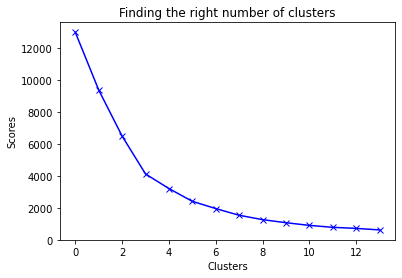
Figure 1 : Number of Clusters
From above graph we can say that the best number of cluster for this is 3 or 4. We will go with 4 numbers of clusters; you can try 3 numbers of clusters also.
    kmeans = KMeans(4)
    kmeans.fit(data_scaled)
    data['cluster'] = kmeans.labels_
    data[data.cluster == 1].head(10)

            Recency  Frequency  Monetary  cluster
CustomerID
12350.0         310          1     25.20        1
12353.0         204          1     19.90        1
12354.0         232          1     20.80        1
12355.0         214          1     30.00        1
12361.0         287          1     23.40        1
12365.0         291          2    335.69        1
12373.0         311          1     19.50        1
12377.0         315          2     57.00        1
12383.0         184          5    102.40        1
12386.0         337          2     98.00        1

    data[data.cluster == 2].head(10)

            Recency  Frequency  Monetary  cluster
CustomerID
12346.0         325          1  77183.60        2
12748.0           0        210   3841.31        2
12971.0           3         86   3952.36        2
13089.0           2         97   5389.39        2
13408.0           1         62   4682.30        2
13694.0           3         50   7519.06        2
13798.0           1         57   8194.26        2
14156.0           9         55   6010.73        2
14527.0           2         55    613.21        2
14606.0           1         93   1023.97        2
sns.boxplot(data.cluster,data.Recency)
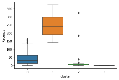
Figure 2 : Recency Distribution as a parameter in Clusters
sns.boxplot(data.cluster,data.Frequency)
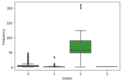
Figure 3 : Frequency Distribution as a parameter in Clusters
sns.boxplot(data.cluster,data.Monetary)
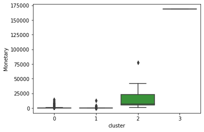
Figure 4 : Monetary Distribution as a parameter in Clusters
Conclusion
A company can get benefits from customer segmentation as it is easy for them to target their customer in more personalized way and do target marketing. With the help of RFM modeling it is easy to do customer segmentation or group them with similar characteristic and business insights can be made. It is helpful in various sectors like financial, marketing, sales, etc. You can read this interesting article on Survival models.
About the Author's:
Write A Public Review